
Why Should I Trust Science If It Can’t Prove Anything?
It’s worth delving a bit deeper into why we ought to trust the scientific inductive process, even when it relies on limited samples that don’t offer absolute “proof.” To do this, let’s examine a widespread practice in psychological science: null-hypothesis significance testing.
To understand this concept, let’s begin with another research example. Imagine, for instance, a researcher is curious about the ways maturity affects academic performance. She might have a hypothesis that mature students are more likely to be responsible about studying and completing homework and, therefore, will do better in their courses. To test this hypothesis, the researcher needs a measure of maturity and a measure of course performance. She might calculate the correlation—or relationship—between student age (her measure of maturity) and points earned in a course (her measure of academic performance). Ultimately, the researcher is interested in the likelihood—or probability— that these two variables closely relate to one another. Null-hypothesis significance testing (NHST)assesses the probability that the collected data (the observations) would be the same if there were no relationship between the variables in the study. Using our example, the NHST would test the probability that the researcher would find a link between age and class performance if there were, in reality, no such link.

Is there a relationship between student age and academic performance? How could we research this question? How confident can we be that our observations reflect reality? [Image: Jeremy Wilburn, https://goo.gl/i9MoJb, CC BY-NC-ND 2.0, https://goo.gl/SjTsDg]
Now, here’s where it gets a little complicated. NHST involves a null hypothesis, a statement that two variables are not related (in this case, that student maturity and academic performance are not related in any meaningful way). NHST also involves an alternative hypothesis, a statement that two variables are related (in this case, that student maturity and academic performance go together). To evaluate these two hypotheses, the researcher collects data. The researcher then compares what she expects to find (probability) with what she actually finds (the collected data) to determine whether she can falsify, or reject, the null hypothesis in favor of the alternative hypothesis.
How does she do this? By looking at the distribution of the data. The distribution is the spread of values—in our example, the numeric values of students’ scores in the course. The researcher will test her hypothesis by comparing the observed distribution of grades earned by older students to those earned by younger students, recognizing that some distributions are more or less likely. Your intuition tells you, for example, that the chances of every single person in the course getting a perfect score are lower than their scores being distributed across all levels of performance.
The researcher can use a probability table to assess the likelihood of any distribution she finds in her class. These tables reflect the work, over the past 200 years, of mathematicians and scientists from a variety of fields. You can see, in Table 2a, an example of an expected distribution if the grades were normally distributed (most are average, and relatively few are amazing or terrible). In Table 2b, you can see possible results of this imaginary study, and can clearly see how they differ from the expected distribution.
In the process of testing these hypotheses, there are four possible outcomes. These are determined by two factors: 1) reality, and 2) what the researcher finds (see Table 3). The best possible outcome is accurate detection. This means that the researcher’s conclusion mirrors reality. In our example, let’s pretend the more mature students do perform slightly better. If this is what the researcher finds in her data, her analysis qualifies as an accurate detection of reality. Another form of accurate detection is when a researcher finds no evidence for a phenomenon, but that phenomenon doesn’t actually exist anyway! Using this same example, let’s now pretend that maturity has nothing to do with academic performance. Perhaps academic performance is instead related to intelligence or study habits. If the researcher finds no evidence for a link between maturity and grades and none actually exists, she will have also achieved accurate detection.
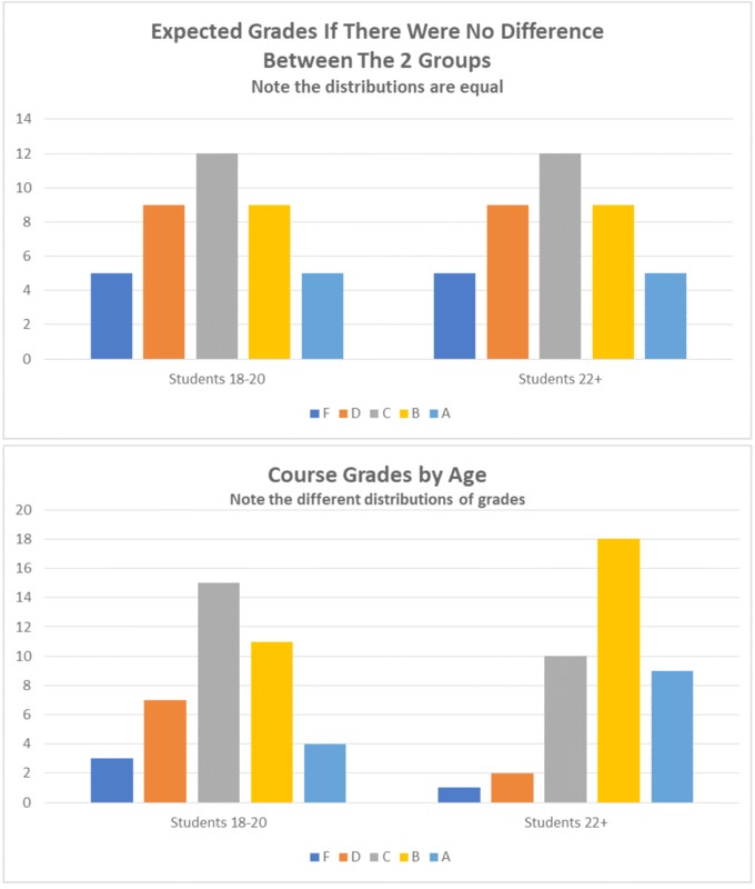
Table 2a (Above): Expected grades if there were no difference between the two groups. Table 2b (Below): Course grades by age
There are a couple of ways that research conclusions might be wrong. One is referred to as a type I error—when the researcher concludes there is a relationship between two variables but, in reality, there is not. Back to our example: Let’s now pretend there’s no relationship between maturity and grades, but the researcher still finds one. Why does this happen? It may be that her sample, by chance, includes older students who also have better study habits and perform better: The researcher has “found” a relationship (the data appearing to show age as significantly correlated with academic performance), but the truth is that the apparent relationship is purely coincidental—the result of these specific older students in this particular sample having better-than-average study habits (the real cause of the relationship). They may have always had superior study habits, even when they were young.
Another possible outcome of NHST is a type II error, when the data fail to show a relationship between variables that actually exists. In our example, this time pretend that maturity is —in reality—associated with academic performance, but the researcher doesn’t find it in her sample. Perhaps it was just her bad luck that her older students are just having an off day, suffering from test anxiety, or were uncharacteristically careless with their homework: The peculiarities of her particular sample, by chance, prevent the researcher from identifying the real relationship between maturity and academic performance.
These types of errors might worry you, that there is just no way to tell if data are any good or not. Researchers share your concerns, and address them by using probability values (p- values) to set a threshold for type I or type II errors. When researchers write that a particular finding is “significant at a p < .05 level,” they’re saying that if the same study were repeated 100 times, we should expect this result to occur—by chance—fewer than five times. That is, in this case, a Type I error is unlikely. Scholars sometimes argue over the exact threshold that should be used for probability. The most common in psychological science are .05 (5% chance), .01 (1% chance), and .001 (1/10th of 1% chance). Remember, psychological science doesn’t rely on definitive proof; it’s about the probability of seeing a specific result. This is also why it’s so important that scientific findings be replicated in additional studies.
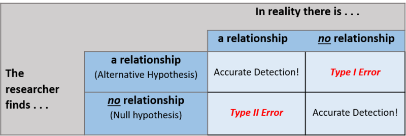
Table 3: Accurate detection and errors in research
It’s because of such methodologies that science is generally trustworthy. Not all claims and explanations are equal; some conclusions are better bets, so to speak. Scientific claims are more likely to be correct and predict real outcomes than “common sense” opinions and personal anecdotes. This is because researchers consider how to best prepare and measure their subjects, systematically collect data from large and—ideally—representative samples, and test their findings against probability.
