
Analysis of Non-Parametric Outcomes
23 Computing the Sign Test
A good place to begin the application of non-parametric statistical applications is with the sign test. Just as the name implies, the sign test is a non-parametric statistical procedure that evaluates the number of differences between paired comparisons using + and – signs to represent the direction of the differences between the pairs.
We can think of the sign test as a statistical method that compares pairs of outcomes and uses the (+) sign to describe the agreement and the (-) sign for the disagreement.
Consider that we wish to compare the number of symptoms reported by concussed patients in two different groups. The first group will be comprised of individuals who are asked to sit quietly in their room for seven days following their concussion injury. The second group will be comprised of individuals that are asked to participate in seven days of controlled and monitored exercise beginning 24 hours after the individual is asymptomatic.
Given this scenario, the sign test can be used to test the null hypothesis in the two-group comparison, where the null hypothesis is written as:
The chance for the number of symptoms in group 1 (the sedentary group) to be greater than the number of symptoms in group 2 (the exercise group) is equal to the chance for the number of symptoms in group 1 (the sedentary group) to be less than the number of symptoms in group 2 (the exercise group).
The numeric value associated with the aforementioned chance is equal to 0.5 or one half and is written as:
$$p(scoregroup1 > scoregroup2) = p(scoregroup1 < scoregroup2) = ½$$
We can simplify the computations of the sign test by evaluating the outcomes using the binomial equation. The binomial equation is a formula that computes exact probabilities for an outcome with two possible options.
In this first example, when comparing symptoms between a patient in group 1 and a patient in group 2, the two possible outcomes are either to have more symptoms or less symptoms.
In the SIGN TEST the outcome options are represented with a (+) or a (-) sign, and as such, the binomial equation can be used to estimate exact probabilities for any pairwise comparison.
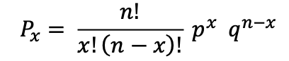
NOTE: The following is a quick overview of the elements of the binomial equation used to establish probability.
Px refers to the probability of exactly x events appearing in n trials. For example – the probability of turning up three heads in 5 tosses of a fair coin.
px refers to the expected probability of the event associated with the x term on any given trial (if we are flipping a coin then this value is ½ with a fair coin).
qn-x refers to the probability of an event on any given trial q = 1- p (usually this value is ½ if we were flipping a coin).
n refers to the number of events.
x refers to the number of a given outcome being evaluated (e.g. how many heads were you expecting in the total number of tosses).
In the application of the sign test, the binomial equation can be used to determine if the number of (+) signs occurs more or less often than the number of (-) signs.
Application 1:
Consider that you are responsible to test the efficacy of exercise treatment for concussion recovery at your rehabilitation clinic. You decide for the next 20 patients that arrive following a concussion, alternate assignment of the patient to either the sedentary group or the activity group. After 7 days of treatment within their respective groups, you survey the patient to determine if the number of symptoms reported by the group assigned to sedentary therapy is higher (or lower) than the number of symptoms reported by the group assigned to the physical activity intervention.
The data are presented in the table below, and the sign test is used to determine if the p(symptom reports in group 1 > symptom reports in group 2) = p(symptom reports in group 1 < symptom reports in group 2) = ½.
In the table, the number of symptoms reported by each pair of members from either the sedentary group or the activity group are compared, and the difference is recorded as being either greater than or less than.
Table of Matched group data example of symptom reporting in exercising versus sedentary patients recovering from concussion.
| Number of Symptoms (Exercise Group) | Number of Symptoms (Sedentary Group) | Comparing Exercise to Sedentary patients | Sign (+) of difference between symptom reports |
| 16 | 19 | < | + |
| 14 | 18 | < | + |
| 18 | 21 | < | + |
| 10 | 09 | > | – |
| 14 | 21 | < | + |
| 16 | 20 | < | + |
| 10 | 08 | > | – |
| 12 | 18 | < | + |
| 08 | 18 | < | + |
| 10 | 20 | < | + |
| 16 | 19 | < | + |
| 14 | 18 | < | + |
| 18 | 21 | < | + |
| 10 | 19 | < | + |
| 14 | 21 | < | + |
| 16 | 20 | < | + |
| 10 | 08 | > | – |
| 12 | 18 | < | + |
| 08 | 18 | < | + |
| 10 | 20 | < | + |
Note: The sign is recorded as (+) when the sedentary group member has more symptoms reported than the matched exercise group member.
These data can be compared using the binomial formula, shown here for a sample of n=20 pairs of patients. In this equation x refers to the number of patients from the sedentary group reporting more symptoms than the patients in the exercise group (x = 17), and the expected probability, based on the null hypothesis where we expected that the number of pairs of patients reporting more or fewer symptoms would be equal is p=0.5.
In the sign test, the test statistic is the number of (+) signs.
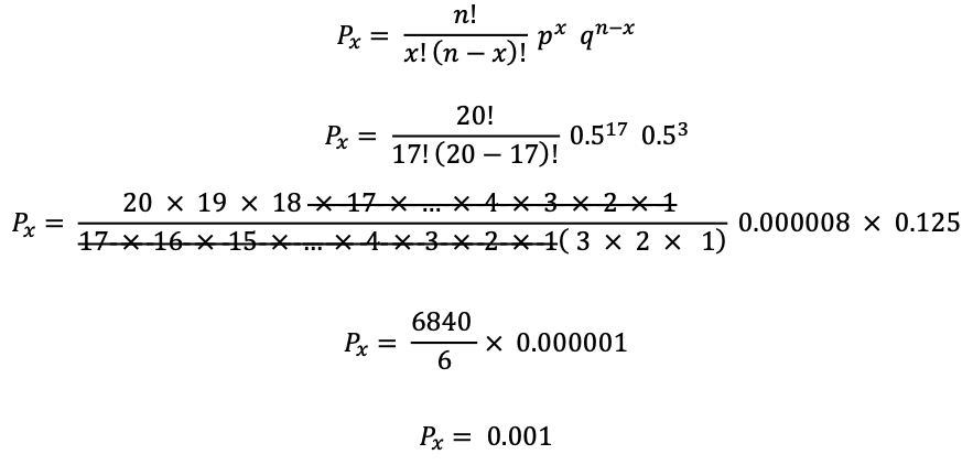
By convention, we typically accept the null hypothesis when the resulting Px is greater than 0.05. In this example where we compared the number of patients from the sedentary group reporting more symptoms than the patients in the exercise group, the probability is 0.001 suggesting that the null hypothesis is false and therefore can be rejected.
In SAS, we can evaluate the null hypothesis for this example using the following program. The problem with the application of the PROC UNIVARIATE procedure here is that the sample size is too small to meet the assumptions of normality and therefore computing the significance of the difference requires that we consider an alternative to the parametric tests. Hence the comparison is an excellent opportunity to consider a non-parametric test like the SIGN-TEST.
SAS program to compute the SIGN TEST using PROC UNIVARIATE
DATA SIGN;
INPUT @1 PAIRNUM EXGRP SEDGRP SIGNPOS;
PAIRDIFF=(SEDGRP-EXGRP);
LABEL EXGRP = “NUMBER OF SYMPTOMS REPORTED BY EXERCISE PATIENT”
SEDGRP = “NUMBER OF SYMPTOMS REPORTED BY SEDENTARY PATIENT”
PAIRDIFF = “DIFFERENCE BETWEEN”
SIGNPOS = “SIGN IS POSITIVE”;
DATALINES;
01 16 19 1
02 14 18 1
03 18 21 1
04 10 09 0
05 14 21 1
06 16 20 1
07 10 08 0
08 12 18 1
09 08 18 1
10 10 20 1
11 16 19 1
12 14 18 1
13 18 21 1
14 10 19 1
15 14 21 1
16 16 20 1
17 10 08 0
18 12 18 1
19 08 18 1
20 10 20 1
;
PROC UNIVARIATE FREQ; VAR PAIRDIFF;
TITLE “COMPUTING THE SIGN TEST FOR PAIRDIFF”;
RUN;
The output table is shown below. The value produced for the sign test shown here is an estimate for a two-tailed test and therefore, the p-value should be divided by 2. Notice that the SAS table produced a p-value of 0.0026 for the two-tailed test which we convert to p=0.001 for a one-tailed test.
Tests for Location: Mu0=0
| Test | Statistic |
p Value |
||
| Student’s t | t | 5.710367 | Pr > |t| | <.0001 |
| Sign | M | 7 | Pr >= |M| | 0.0026 |
| Signed Rank | S | 99 | Pr >= |S| | <.0001 |
The information that is relevant from the SAS output produced above is the SIGN Test result Pr >=|M| (0.0026/2)=0.001. This result indicates that there is a significant difference in the responses of the two groups as determined by the SIGN test.
Application 2:
Consider that you have two samples of 10 individuals in each sample. You identify a group of 10 smokers and a matched group of 10 non-smokers — and you are interested in determining if the outcome on the dependent measure (resting heart rate) is the same in both groups. You begin by matching the participants in your groups on the variables: age, sex, socio-economic status, education, and smoking status where you separate the groups according to: never smoked versus smoke at least 3 cigarettes per day. Then you measure the resting heart rate for individuals after asking them to sit quietly for 5 minutes (without smoking!!).
Table of matched group data example of smokers versus non-smokers with the outcome heart rate (bpm)
| Non-smoker heart rate (bpm) | Smoker heart rate (bpm) | Compare Non-Smoker to Smoker | Sign (+) when NShr < Shr |
| 76 | 99 | < | + |
| 54 | 78 | < | + |
| 68 | 68 | tied | tied |
| 60 | 54 | > | – |
| 54 | 82 | < | + |
| 86 | 92 | < | + |
| 90 | 80 | > | – |
| 62 | 78 | < | + |
| 58 | 88 | < | + |
| 60 | 90 | < | + |
Notice in the table above there are 7 occurrences where the heart rate measures for non-smokers showed fewer beats per minute than the smokers. Notice also that there was one occurrence in which the heart rate for the smoker was the same as the heart rate for the non-smoker. In the SIGN test, the number of ties is not included in the binomial computation.
Applying the binomial formula for computations in the Sign-Test
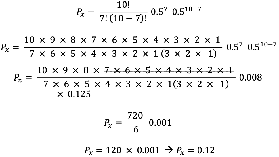
In our sample data to compare heart rates in smokers versus non-smokers for n=10, x=7, p=0.5 and q=0.5 we begin by applying the binomial formula.
To test the difference in heart rates we counted the number of times that non-smokers’ heart rates were lower than smokers’ heart rates. Our count was 7 out of 10, and the probability of observing 7 out 10 in any random selection of smokers and non-smokers, matched on age, sex, socio-economic status, education, and smoking group where the groups were separated according to: never smoked versus smoke at least 3 cigarettes per day was found to be Px = 0.12. The arithmetic is shown below:
Recall that when evaluating the null hypothesis: H0: Group1 = Group2 we can use the standard normal distribution. We generally accept the null hypothesis when the probability associated with the difference between our estimates is less than 0.05.
Therefore, we conclude from these data that the two groups are equal for their resting heart rates.
However if the number of times we observed a non-smoker’s heart rate to be less than a smoker’s resting heart rate was 8 times ( or 8 out of the 10 participants) then the value of Px would have been Px =0.043 and by convention we would have said that there was a difference in resting heart rates in this sample of smokers and non-smokers.
