| Parameter Estimates for Figure 33.1 | |||||||
|---|---|---|---|---|---|---|---|
| Variable | DF | Parameter Estimate |
Standard Error |
t Value | Pr > |t| | 95% Confidence Limits | |
| Intercept | 1 | 22.40 | 0.916 | 24.44 | <.0001 | 20.29 | 24.51 |
| trial | 1 | 2.60 | 0.147 | 17.60 | <.0001 | 2.26 | 2.94 |
Parametric Statistics
33 Statistical applications with linear regression analyses
Learner Ootcomes
After reading this chapter you should be able to:
- Define and describe simple linear regression
- Create a SAS program to compute the outcome for a linear regression application including the slope of a line
- Create a line of best fit
- Identify the critical components in the output generated from a linear regression application
Calculating the slope of a line
The first step in understanding linear regression is to review the calculation for the slope of a line.
Although presented early in your introduction to mathematics and algebra, most likely in secondary school, learning about the slope of a line may have been one of those topics that you missed, or forgot, or decided that you would never need in the future. Of course, since your intended vocation was not going to require statistical analyses and only essential math, why bother listening. However, now we are reviewing statistical applications and so understanding the calculation for the slope of a line is actually meaningful.
Providing an estimate for the slope of a line can be one way to calculate the rate of change in a variable of interest on the vertical axis – usually denoted as y, in relation to an independent variable, such as time plotted on the horizontal axis – denoted as x. The slope of a line provides a measure of the steepness of the line as a function of the change in the variable (y) in relation to the change in the variable (x). Consider for example the data plotted in the following graph (Figure 33.1).
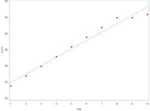
Figure 33.1 Line of Best fit or Y (Score) over X (Time)
In the graph above, we observe a distinct positive relationship between the scores for the variable on the y-axis and the scores for the variable on the x-axis. That is, as we move from left to right on the x-axis we observe an increase in the scores on the y-axis. The slope of the line is an estimate or what we refer to as a coefficient, a single number that represents all of the points on the line of the relationship between the variables: x and y.
The basic calculation to determine this estimate (i.e. the slope) of this relationship is given here as [latex]slope = {\Delta{y}\over\Delta{x}}[/latex] which is read as the change in the y variable divided by the change in the x variable.
Key Takeaways
The slope of a straight line is constant for the entire line and therefore any two points, chosen at random on the line will provide the estimate of the slope (this is not the case for non-linear lines). You might recall that the slope of a line is often represented by the letter m, and the formula for slope is read as: slope = rise over run.
Using SAS programming as shown below, we see that The slope of the line for the graph above is 2.60, and the y-intercept (the point where the line crosses the y-axis) is 22.40. Both estimates are shown in the table below.
Determining the Slope of a line
The SAS code for the graph above is shownhere. The program uses two variables: the independent variable (x) called TRIAL and the outcome variable (y) called SCORE. Lines 1 to 3 in the code below set up the program environment. Line 4 identifies the program workflow. Line 5 explains the arrangement of the columns of data. Line 6 cues the program that the data will follow. Ten data points are included in this dataset. Lines 7 to 16 are the SAS code to produce the regression estimates and create the graph with both a line and with dots to represent each point.
-
options pagesize=55 linesize=120 center date;
-
goptions reset=all cback=white border htitle=12pt htext=10pt;
-
LIBNAME txtbook '/home/username/textbookExamples/regression';
-
data txtbook.slope1;
-
input trial 1-2 score 4-5;
-
datalines;
01 24
02 27
03 30
04 33
05 36
06 39
07 42
08 45
09 45
10 46
;
-
Title 'Estimating the slope';
-
axis1 label=("Trial"); axis2 label=(angle=90 "Score") minor=(n=4); /* Define the symbol characteristics for the plot groups */ -
symbol1 interpol=none value=dot color=depk;
-
symbol2 interpol=none value=dot color=vibg;

/* Define the symbol characteristics for the regression line */
-
symbol3 interpol=rl value=none color=black;

/* proc gplot data=txtbook.slope1;
-
plot score*trial / haxis=axis1 vaxis=axis2 ;
-
plot2 score*trial / noaxis; */
-
proc reg; model score=trial / clb; /* command to produce estimates */
-
plot score*trial ="*";
-
run;
Let’s consider a research application of simple linear regression. In the following research study, we are interested in the change in pain estimates for horses that undergo castration. Here we collected 4 pain estimates at 30-minute intervals following equine castration surgery. The data for the estimates of pain are represented in the following table. Notice for each 30-minute time point the estimate of pain on a 10 point scale diminishes by one point.
| Time in reference to surgery | 30 minutes after | 60 minutes after | 90 minutes after | 120 minutes after |
| 10-point pain scale | 9 | 8 | 7 | 6 |
We can graph these data using the following SAS code.
Example 33.2 Application of Simple Linear Regression
DATA LINE;
INPUT ID TIME PAIN;
DATALINES;
01 30 9
02 60 8
03 90 7
04 120 6
;
PROC SGPLOT NOBORDER NOAUTOLEGEND;
REG Y=PAIN X=TIME;
RUN;
Figure 33.2, below shows the line of best fit that illustrates the relationship between pain ratings over time since surgery.
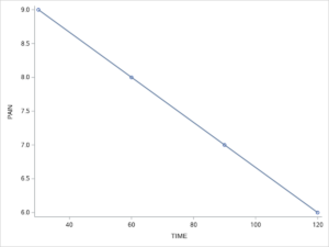
Figure 33.2. Pain Ratings Following Surgery
The calculation of the slope of the line for the estimate of pain over time is represented by the following equation.
[latex]slope = {\Delta{y}\over\Delta{x}}[/latex]
[latex]slope = {(y_2 - y_1)\over (x_2 - x_1)} =[/latex]
[latex]slope = {(8 - 9)\over (60 - 30)} = {(-1)\over (30)} ={0.033}[/latex]
Notice that the slope has a value of m -0.033 which when multiplied by the time value in the equation [latex]y = {mx + b}[/latex] indicates that as the value of TIME increases from left to right on the x-axis, the value for PAIN decreases on the y-axis.
With the following lines of SAS code added to our program we can compute the slope and the y-intercept term for the data above and cofirm that which we calculated by hand.
PROC REG; MODEL PAIN = TIME;
RUN;
This SAS code produced the following output.
The REG Procedure — Model: MODEL1 for Dependent Variable (Y) : pain
| Parameter Estimates | |||||
| Variable | DF | Parameter Estimate |
Standard Error |
t Value | Pr > |t| |
| Intercept | 1 | 10.00000 | 0 | Infty | <.0001 |
| time (x variable) |
1 | -0.03333 | 0 | -Infty | <.0001 |
Notice both the slope score of -0.033 and the y-intercept (10) are included in this table. Likewise, because there are only four scores in the data set the standard error is 0 and the estimates for slope and y-intercept are significantly greater than 0.
Using Regression to Compute a Laboratory Standard Curve
In many laboratory experiments, researchers will create what is known as a curve of standards or a standard curve to establish the relationship between substrates and products.. One way that we can use regression and the calculation of the line of best fit is to test the linearity of a relationship between the concentrations of a substrate (x) and a product (y). In the following example we were measuring the presence of a gene of interest at 5 different concentrations.
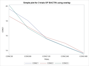
The Gene of interest was Bactin and the concentrations were: EXPAND..
The following SAS program was used to calculate the relationship using regression, and the graphical representation of the relationship.
SAS progran to compute line of best fit with PROC REG & PROC SGPLOT
PROC FORMAT;
VALUE TRFMT 1=’CONC30′
2=’CONC60′
3=’CONC120′
4=’CONC240′
5=’CONC480′;
options pagesize=55 linesize=80 center;
LIBNAME LINES20 ‘/home/username/bioInfomatics/lnBstFt’;
DATA LINES20.BACTIN01;
input TRIAL CONC1 CONC2 CONC3;
DATALINES;
1 19.63 18.63 20.12
2 18.06 17.23 17.05
3 15.63 15.80 15.59
4 14.58 15.00 14.57
5 13.64 13.70 13.56
;
proc reg;
model CONC1=TRIAL;
model CONC2=TRIAL;
model CONC3=TRIAL;
run;
proc sgplot data=LINES20.BACTIN01
noautolegend;
reg x=TRIAL y=CONC1 / CLM
CLMATTRS=(CLMLINEATTRS=
(COLOR=Green PATTERN= ShortDash));
FORMAT TRIAL TRFMT. ;
TITLE ‘ CONFIDENCE LIMITS FOR TRIAL 1 OF BACTIN’;
run;
proc sgplot data=LINES20.BACTIN01
noautolegend;
reg x=TRIAL y=CONC2 / CLM
CLMATTRS=(CLMLINEATTRS=
(COLOR=Green PATTERN= ShortDash));
FORMAT TRIAL TRFMT. ;
TITLE ‘ CONFIDENCE LIMITS FOR TRIAL 2 OF BACTIN’;
run;
proc sgplot data=LINES20.BACTIN01
noautolegend;
reg x=TRIAL y=CONC3 / CLM
CLMATTRS=(CLMLINEATTRS=
(COLOR=Green PATTERN= ShortDash));
FORMAT TRIAL TRFMT. ;
TITLE ‘ CONFIDENCE LIMITS FOR TRIAL 3 OF BACTIN’;
run;
proc sgplot data=LINES20.BACTIN01;
xaxis type=discrete;
series x=TRIAL y=CONC1;
series x=TRIAL y=CONC2;
series x=TRIAL y=CONC3;
;
FORMAT TRIAL TRFMT. ;
TITLE ‘ Simple plot for 3 trials OF BACTIN using overlay’;
run;
Output from PROC REG
The REG Procedure
Model: MODEL3
Dependent Variable: CONC3
| Number of Observations Read | 5 |
|---|---|
| Number of Observations Used | 5 |
| Analysis of Variance | |||||
|---|---|---|---|---|---|
| Source | DF | Sum of Squares |
Mean Square |
F Value | Pr > F |
| Model | 1 | 24.33600 | 24.33600 | 41.74 | 0.0075 |
| Error | 3 | 1.74908 | 0.58303 | ||
| Corrected Total | 4 | 26.08508 | |||
| Root MSE | 0.76356 | R-Square | 0.9329 |
|---|---|---|---|
| Dependent Mean | 16.17800 | Adj R-Sq | 0.9106 |
| Coeff Var | 4.71975 |
| Parameter Estimates | |||||
|---|---|---|---|---|---|
| Variable | DF | Parameter Estimate |
Standard Error |
t Value | Pr > |t| |
| Intercept | 1 | 20.85800 | 0.80083 | 26.05 | 0.0001 |
| TRIAL | 1 | -1.56000 | 0.24146 | -6.46 | 0.0075 |