
Parametric Statistics
27 Measures of Variance
PART 2: Measures of Variance
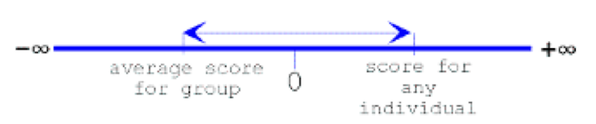
In quantitative methods, we are often interested in the spatial relationship between responses within a set of numbers. We can describe this relationship as the dispersion of scores around the mean, or state that the dispersion of scores is represented by the variability or variance of the scores around the mean. For example, consider a straight line with boundaries at negative infinity and positive infinity. Notice that the straight line is continuous between the two boundary points, and within this space, we can measure the distance between an individual’s score and the estimated average score of a group of scores.
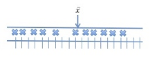
The differences between each observed score and the mean score within a set of scores are referred to as the variability of scores. In the following three images we can see the relationship between scores within a distribution and the mean of the distribution. In the first image, shown below, the scores – represented by X – are plotted on a scale from lowest to highest, and the algebraic midpoint is shown as the mean ([latex]\overline{x}[/latex]).
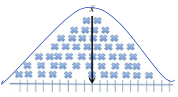
In the second image, we see the mean for the distribution is included in the image as a reference point to show the algebraic center of the distribution. In this second figure, we see the accumulation of all scores in the set of data. Notice how they create a shape for the distribution.
If we drew a smooth line over the top of this pile of scores it may indicate a bell shape.
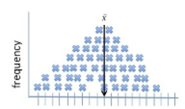
In the third image, we see the scale of the frequency of the scores within the distribution is added to the left side of the image. The Y-axis is labeled frequency and can provide a count of scores at each of the values on the x-axis. The frequency is used to compute the proportion of scores within the entire set of scores.
Since we have a set of data, we can compute both the measure of centrality (the mean) as well as the average distance between the individual scores and the estimated mean. The average distance of scores from the mean is referred to as the variance.
Calculating Variance
Although we can conceptualize variance as an average score, this average score is not simply calculated by summing the difference scores and dividing by the number of scores. Rather, the variance score can be calculated for a “population” and for a “sample”, where the terms in the denominators of the two calculations differ. The formulas to compute variance, first for a population and then for a sample are shown in the following two equations, below. Notice that the variance for the population is the average squared difference between the scores and the mean [latex]\mu[/latex]. However, in the calculation of variance for the sample, we subtract 1 in the denominator to enable us to produce an estimate which will be large enough to capture the true population estimate.
i) Population Variance: [latex]\sigma^2 = {{\sum(x_{i}- \mu)^2 \over {N}}}[/latex]
ii) Sample Variance: [latex]s^2 = {{\sum(x_{i}- \overline{x})^2 \over {n - 1}}}[/latex]
Standard Deviation
The term deviation refers to differences. When we consider deviation in a sample or a set of scores we are really interested in the dispersion of the scores around the mean. The term standard deviation refers to the “standardized estimate of variance”. The standard deviation presents the variance in the original units of measurement.
The standard deviation is derived from the estimate of variance and is computed by calculating the square root of the variance as shown in equation iii) – standard deviation for a population and equation iv) – standard deviation for a sample, as shown below.
iii) Population Standard Deviation: [latex]\sigma^2 = {\sqrt{{\sum(x_{i}- \mu)^2 \over {N}}}}[/latex]
iv) Sample Standard Deviation: [latex]s^2 = {\sqrt{{\sum(x_{i}- \overline{x})^2 \over {n - 1}}}}[/latex]
In quantitative methods, we often consider the spreads of distributions and the shape of distributions. Estimates of difference between an individual’s score and the measure of central tendency, the shape of the distribution, and the size of the distribution, are all elements of VARIANCE.
The Coefficient of Variation
We use the coefficient of variation to compare the dispersion of scores around the mean. The coefficient of variation is computed by dividing the standard deviation by the mean and multiplying by 100, as shown in equation v).
v) Coefficient of Variation: [latex]cv = {s \over {\overline{x}}} \times 100[/latex]
The coefficient of a variation is a useful measure to show the dispersion of a sample of scores around the mean. When used as a single measure it may not be as effective as when it is used as a comparative measure between two samples. The coefficient of variation is an effective measure to compare data from different samples. In the following example, we demonstrate the usefulness of the coefficient of variation by comparing the spread of scores around the mean in two samples measuring systolic blood pressure at rest. Here we recorded resting systolic blood pressure measures for a sample of males and a sample of females in a graduate course in biostatistics. The SAS program to compute the coefficient of variation for the comparison is shown in the example below.
SAS program to compute the coefficient of variation
DATA SPREAD;
INPUT ID GRP SCORE @@;
DATALINES;
01 1 121 02 1 134 03 1 133
04 1 128 05 1 125
06 1 127 07 1 124 08 1 123
09 1 126 10 1 128
11 2 134 12 2 156 13 2 129
14 2 141 15 2 142 16 2 139 17 2 138
18 2 145 19 2 133 20 2 145
;
PROC SORT DATA=SPREAD; BY GRP;
PROC MEANS N MEAN STDDEV MEDIAN MODE CV;
VAR SCORE; BY GRP;
RUN;
Output from the SAS MEANS Procedure
| Analysis Variable: SCORE for GRP=1 | |||||
| N | Mean | Std Dev | Median | Mode | Coeff of Variation |
| 10 | 126.90 | 4.12 | 126.50 | 128.00 | 3.25 |
| Analysis Variable: SCORE for GRP=2 |
|||||
| N | Mean | Std Dev | Median | Mode | Coeff of Variation |
| 10 | 140.20 | 7.61 | 140.00 | 145.00 | 5.43 |
Notice in the comparison of the scores in the two groups above, the mean for group 1 was 126.9 with a standard deviation of 4.12. In group 2, the mean score was 140.2 with a standard deviation of 7.61. These scores indicate that group 1 had less dispersion of scores around the mean (C.V. = 3.25), while group 2 had a much larger spread of scores around the mean (C.V. = 5.43). We can interpret these data to say that the data in group 2 was less homogenous than the data for group 1.
PART 3: Shapes of Distributions
Skewness
Skewness is an estimate of variability and as such, skewness is considered the “third moment” of scores within a distribution. This is easily recognized in the formula for skewness shown below.
Skewness: [latex]skew = {{\sum(x_{i}- \overline{x})^3 \over {N}}}[/latex]
The estimate of skewness is the ratio of the sum of the cubed differences between the observed scores and the mean to the number of scores in the sample. Unlike variance, which squared the difference scores, skewness computes the cube of the difference scores. That is, skewness is computed by:
- subtracting each observation from the average score,
- raising the difference to the exponent “3”,
- summing the cubes and then
- dividing by the number of observations (or the number of observations minus one).
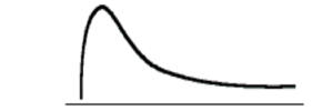
A negative skewness score indicates a negatively skewed distribution, while a positive skewness score indicates a positively skewed distribution. Examples of skewed distributions are shown below.
Illustration of negative skewness shown here — notice the tailing off of the distribution toward negative infinity.
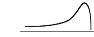
Illustration of a normal distribution (no skewness) — notice the symmetry of the distribution, there is no tailing-off toward either negative or positive infinity.
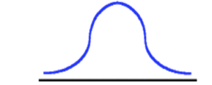
Illustration of positive skewness — notice the tailing off of the distribution toward positive infinity
In most applications, the raw skewness is not used. Rather the reader is directed to the “standardized skewness” as shown in the formula presented in the equation, below.
Standardized Skewness: [latex]skew = {{\sum(x_{i}- \overline{x})^3 \over {N}}} \times({ 1\over {s^2 *s}})[/latex]
Kurtosis
Kurtosis is also an estimate of variability. Kurtosis is considered the “fourth moment” of scores within a distribution. Again, this is easily recognized by the formula for kurtosis shown in the equation below. Notice that similar to estimates of variance and skewness, the estimate of kurtosis is computed as a ratio of the difference between the observed scores and the mean scores raised to an exponent – in the case of kurtosis the exponent is 4.
[latex]kurtosis = {{\sum(x_{i}- \overline{x})^4 \over {N}}}[/latex]
However, unlike variance, in which the difference scores were squared, and skewness, in which the difference scores were cubed, kurtosis computes the difference scores to the 4th power. That is, kurtosis is computed by:
- subtracting each observation from the average score,
- raising the difference to the exponent “4”,
- summing the products and then
- dividing by the number of observations (or the number of observations minus one).
Examples of kurtosis are shown here:
![]()
The figure above is an illustration of a platykurtic distribution. Notice the flatness of the distribution (remember the term platy refers to flat). In order to achieve a platykurtic distribution, all scores within the distribution are unique. Below is an illustration of the mesokurtic distribution.
Notice in the mesokurtic distribution the shape is that of a normal distribution — neither flat nor demonstrating any peakedness in the distribution. Below is an image illustrating the leptokurtic distribution.
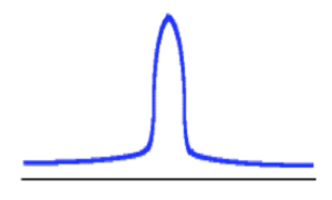
Notice the peak-ness of the distribution (remember the term lepto refers to leaping). In order to achieve a leptokurtic distribution, all scores within the distribution are located close to the mean. There is very little deviation of scores from the measure of the central tendency within the distribution.
In most applications, the raw kurtosis is not used. Rather the reader is directed to the “standardized kurtosis” as shown in the equation below.
Standardized Kurtosis =[latex]{{\sum(x_{i}- \overline{x})^4 \over {N}}} \times({ 1\over {s^2 * s^2}})[/latex]
When computing the standardized skewness and standardized kurtosis a check of the distribution characteristics are as follows:
- When a negative skewness value is observed, the distribution is negatively skewed. (tailing to the negative – the left)
- When a positive skewness value is observed, the distribution is positively skewed. (tailing to the positive – the right)
- When a skewness value is zero, the distribution has no skewness.
- When a kurtosis value is less than three, the distribution is platykurtic.
- When a kurtosis value is greater than three, the distribution is leptokurtic.
- When a kurtosis value is equal to three, the distribution is mesokurtic.
