
Parametric Statistics
31 The One Way Analysis of Variance and Post Hoc Tests
Learner Outcomes
After reading this chapter you should be able to:
- Compute the significance of the difference between three or more sample means using the one way analysis of variance test
- Compute the post-hoc pairwise comparison between sample means when the F statistic is significant
- Write a SAS program to compute and identify the important elements of the output for the computation of the one-way analysis of variance
31.1 Analysis of Variance
We use the analysis of variance (ANOVA) to evaluate tests of hypothesis for differences between two or more treatments. In computing the significant difference between multiple means using the One Way Analysis of Variance – ANOVA along with post hoc tests we compare estimates of variance between and within each of the sample groups. The purpose of the ANOVA is to decide whether the differences in the estimates of variance between the samples are simply due to random error (sampling errors) or whether there are systematic treatment effects that have caused scores in one group to differ from scores in another.
In the one-way analysis of variance (ANOVA), we are only comparing the mean scores from three or more samples on one dimension, such as between each group, as shown in the following diagram.
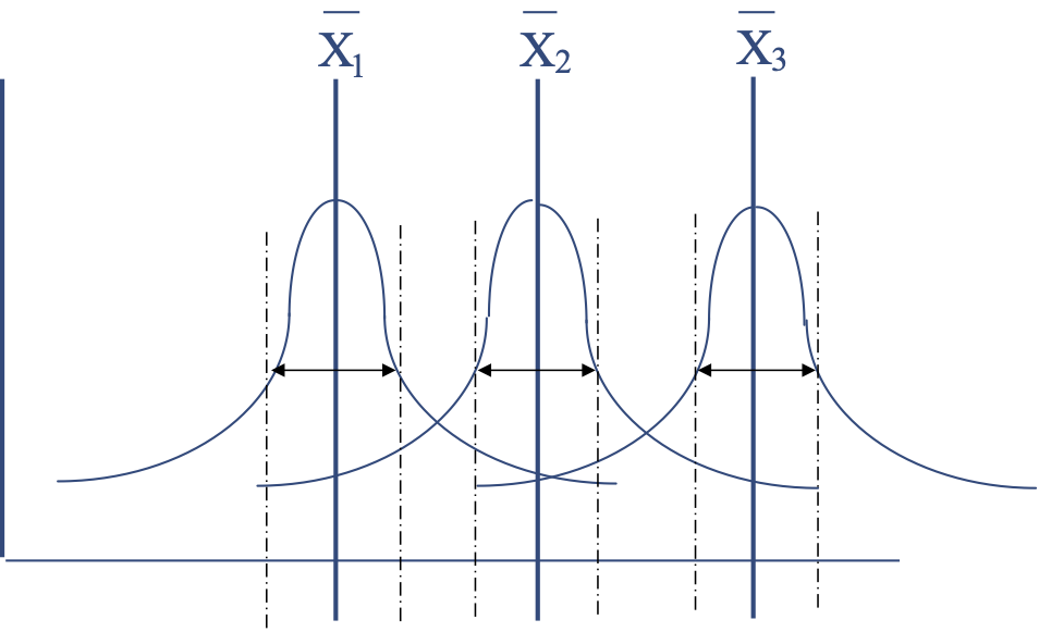
Illustration of the Comparison of Means in the One-way ANOVA
The one-way ANOVA evaluates the variance between samples, and tests the null hypothesis: [latex]H_{0}: \mu_{1} = \mu_{2} = \mu_{k}[/latex], or that [latex]H_{0}: \mu_{1} - \mu_{2} - \mu_{k} = 0[/latex]. The statistic that we use to test this null hypothesis is an F test (producing an F value) and is based on the ratio of the variance between the samples divided by the variance within the samples, as shown here: F = variance between samples / variance within samples
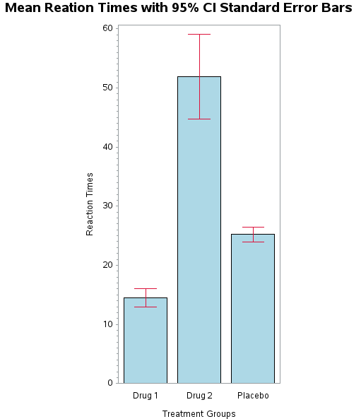
Consider an experiment intended to compare the effects of two independent drugs and placebo on an individual’s reaction time. Here we can define reaction time as the speed at which an individual demonstrates a response to a given stimulus).
This experimental design would require us to create three groups of participants, in which each group consists of individuals that are randomly selected from a population and randomly distributed to one of the groups (drug group 1, drug group 2, or placebo).
The purpose of the experiment would be to determine if there is a significant difference in the measured reaction times for the individuals in each of the drug groups versus individuals in the placebo group.
The data sets are based on the observed reaction times measured for individuals from the two independent drugs and the group that received the placebo. The data are arranged to have 3 groups of 10 individuals per group, wherein each individual within each group provides reaction time measurements. The hypothetical data for this experiment are shown in Table 31.1, below.
Table 31.1 Reaction Time Data for Each Experimental Group
| Reaction time scores recorded in seconds
Group 1: Drug A |
Reaction time scores recorded in seconds
Group 2: Drug B |
Reaction time scores recorded in seconds
Group 3: Placebo |
| 12 | 45 | 25 |
| 15 | 54 | 26 |
| 16 | 39 | 28 |
| 13 | 65 | 22 |
| 14 | 34 | 26 |
| 15 | 63 | 27 |
| 17 | 55 | 23 |
| 11 | 51 | 26 |
| 18 | 53 | 24 |
| 14 | 60 | 25 |
| Sum1 = 145 | Sum2 = 519 | Sum3 = 252 |
A vertical bar chart of the data in Table 31.1 shows an obvious difference in the mean reaction times for each treatment group (Drug1, Drug2, and Placebo). Given the observed difference between means, it is appropriate to test the statistical significance of this difference using a one-way ANOVA.
31.2 Computing the ANOVA by hand
In this experiment, we can calculate the ANOVA by hand to illustrate the essential calculations that are used to produce the F statistic. After we compute the Fobserved we next compare the F observed value to the Fcritical value of 3.35 to determine if we accept or reject H0. The Fcritical value is derived from a table of critical values which we can retrieve from the Internet, and is based on the number of elements (participants) in each group being compared [latex]\rightarrow[/latex] the degrees of freedom.
We begin our calculations by computing the grand mean. The grand mean is the average for all numbers within the entire set of numbers, and is therefore the sum of all scores divided by N (the number of scores) as shown here:
[latex]\overline{X}= \frac{\Sigma{x}_{i}} {N}[/latex] = ((12 + 15 + 16 + 13 + 14 + 15 + 17 + 11 + 18 + 14 + 45 + 54 + 39 + 65 + 34 + 63 + 55 + 51 + 53 + 60 + 25 + 26 + 28 + 22 + 26 + 27 + 23 + 26 + 24 + 25) / N )
[latex]\overline{X}= \frac{\Sigma{x}_{i}} {N}[/latex] =((916)/30) = 30.53
Once we calculate the grand mean, then we are ready to calculate the specific elements of the one way ANOVA. Our next step is then to calculate the Sum of Squares Total ([latex]SS_{total}[/latex]).
The [latex]SS_{total}[/latex] is calculated by calculating the squared difference of each score from the grand mean and summing the difference scores, as shown here:
[latex]SS_{total}= \Sigma\left(x_{ij} - \overline{X}\right)^2[/latex] = ((12-30.53)2+(15-30.53)2+(16-30.53)2+(13-30.53)2+(14-30.53)2+(15-30.53)2+(17-30.53)2+(11-30.53)2+(18-30.53)2+(14-30.53)2+(45-30.53)2+(54-30.53)2+(39-30.53)2+(65-30.53)2+(34-30.53)2+(63-30.53)2+(55-30.53)2+(51-30.53)2+(53-30.53)2+(60-30.53)2+(25-30.53)2+(26-30.53)2+(28-30.53)2+(22-30.53)2+(26-30.53)2+(27-30.53)2+(23-30.53)2+(26-30.53)2+(24-30.53)2+(25-30.53)2
[latex]SS_{total}= \Sigma\left(x_{ij} - \overline{X}\right)^2[/latex] = 343.36 + 241.18 + 211.12 + 307.3 + 273.24 + 241.18 + 183.06 + 381.42 + 157 + 273.24 + 209.38 + 550.84 + 71.74 + 1188.18 + 12.04 + 1054.3 + 598.78 + 419.02 + 504.9 + 868.48 + 30.58 + 20.52 + 6.4 + 72.76 + 20.52 + 12.46 + 56.7 + 20.52 + 42.64 + 30.58
[latex]SS_{total}= \Sigma\left(x_{ij} - \overline{X}\right)^2[/latex] = 8403.44
Our next step is to compare the [latex]SS_{between}[/latex] terms (sometimes referred to as the sum of squares for the treatment term), which is a comparison of the variance in Group 1 against the variance in Group 2 and concomitantly agaist the variance in Group 3.
This is represented as: [latex]S_{1}^2 + S_{2}^2 +S_{3}^2[/latex]
To calculate the between groups sums of squares we subtract each of the individual means [latex]\left( \overline{x}_{j}\right)[/latex] from the grand mean [latex]\left(\overline{X}\right)[/latex] and square the difference scores [latex]\left(\Delta\right)^2[/latex]. We then multiply the squared difference score by the number of participants in each group,) as shown here:
[latex]SS_{between} = \Sigma{n}_{j} \left(\overline{xj} - \overline{X}\right)^2[/latex]
[latex]SS_{between} = \left(10 \times \left(14.5-30.53\right)^2 + 10 \times \left(51.9-30.53\right)^2 + 10 \times \left(25.2 – 30.53\right)^2\right)[/latex]
[latex]SS_{between}[/latex] = (2569.60 + 4566.80 + 284.10) = 7420.49
The error term is calculated from the squared deviations of each of the scores from the mean score within each group. The term [latex]SS_{error}[/latex] is also referred to as the [latex]SS_{within}[/latex] and is shown here.
[latex]SS_{within}[/latex] = \left(\Sigma{x}_{ij} – \overline{x}_{j} \right)^2[/latex]
[latex]SS_{within} \textit{(Group 1)}[/latex] = (12-14.5)2 + (15-14.5)2 + (16-14.5)2 + (13-14.5)2 + (14-14.5)2 + (15-14.5)2 + (17-14.5)2 + (11-14.5)2 + (18-14.5)2 + (14-14.5)2
[latex]SS_{within} \textit{(Group 1)}[/latex] = 6.25 + 0.25 + 2.25 + 2.25 + 0.25 + 0.25 + 6.25 + 12.25 + 12.25 + 0.25
[latex]SS_{within} \textit{(Group 1)}[/latex] = 42.25
[latex]SS_{within} \textit{(Group 2)}[/latex] = (45-51.9)2 + (54-51.9)2 + (39-51.9)2 + (65-51.9)2 + (34-51.9)2 + (63-51.9)2 + (55-51.9)2 + (51-51.9)2 + (53-51.9)2 + (60-51.9)2
[latex]SS_{within} \textit{(Group 2)}[/latex] = 47.61 + 4.41+ 166.41+ 171.61 + 320.41 + 123.21 + 9.61 + 0.81 + 1.21 + 65.61
[latex]SS_{within} \textit{(Group 2)}[/latex] = 910.90
[latex]SS_{within} \textit{(Group 3)}[/latex] = (25-25.2)2 + (26-25.2)2 + (28-25.2)2 + (22-25.2)2 + (26-25.2)2 + (27-25.2)2 + (23-25.2)2 + (26-25.2)2 + (24-25.2)2 + (25-25.2)2
[latex]SS_{within} \textit{(Group 3)}[/latex] = 0.04 + 0.64 + 7.84 + 10.24 + 0.64 + 3.24 + 4.84 + 0.64 + 1.44 + 0.04
[latex]SS_{within} \textit{(Group 3)}[/latex] = 29.6
[latex]SS_{within}[/latex] = (42.25 + 910.90 + 29.6) = 983
The mean square term for the analysis of variance, also known as the mean square between (MSb), is calculated from the sum of squares between divided by the degrees of freedom for that term, as shown below. In this example there were 3 groups therefore the degrees of freedom between groups is (k -1= 3 -1 = 2).
[latex]MS_{b} = \frac {7420.47} {2}[/latex] = 3710.23
Likewise, the mean square for the error term, also referred to as the mean square within (MSw) is calculated by dividing the sum of squares from the error statement [latex]SS_{within}[/latex] = 983, shown above, by the degrees of freedom from the error statement (dferror = dfw = 30 participants – 3 groups = 27). The degrees of freedom for the error term is based on the construct that in this example there were 30 participants in total and three groups, therefore we subtract 1 participant per group from the grand total. Therefore, our degrees of freedom for the MSw term is N-k = 30-3 = 27.
[latex]MS_{w} = \frac {983.00} {27}[/latex] = 36.41
The F- statistic is then calculated by dividing the mean square between by the mean square within, as shown here.
[latex]F_{observed} = \frac {MS_{b}} {MS{_w}} = \frac {3710.23} {36.41}[/latex] = 101.91
In this experiment we computed the F statistic using a one-way analysis of variance—ANOVA. In this scenario we calculated an observed F statistic, also referred to as the [latex]F_{observed}[/latex] of 101.91. Below we explain how to compare an [latex]F_{observed}[/latex] score to an [latex]F_{expected}[/latex], or an [latex]F_{critical}[/latex] value.
31.3 Creating the SAS PROC ANOVA program
The task of applying the ANOVA to these data is to test the null hypothesis that the means of each group are equal. We create a decision rule to evaluate in which we state that: If F observed is greater than F critical then we will reject H0; else if F observed is less than or equal to F critical then we will accept H0 (the null hypothesis).
In the following example, we begin by evaluating the observed or perceived difference between the means using the F statistic from the ANOVA, and the F statistic generated by the PROC GLM procedure of SAS, for the data presented above. The PROC ANOVA and the PROC GLM produce similar output, however, we use the PROC ANOVA term when the number of observations within each group is the same, and we use the PROC GLM procedure when there are a different number of observations in each of the groups being compared. Regardless of whether you choose the PROC ANOVA or the PROC GLM, they both use an F test to evaluate the null hypothesis that there is no difference between means.
SAS for OneWay Anova
DATA ONEWAY1;
INPUT ID GROUP SCORE @@;
DATALINES;
001 01 12 002 01 15 003 01 16 004 01 13 005 01 14 006 01 15
007 01 17 008 01 11 009 01 18 010 01 14 011 02 45 012 02 54
013 02 39 014 02 65 015 02 34 016 02 63 017 02 55 018 02 51
019 02 53 020 02 60 021 03 25 022 03 26 023 03 28 024 03 22
025 03 26 026 03 27 027 03 23 028 03 26 029 03 24 030 03 25
;
PROC SORT DATA=ONEWAY1; BY GROUP;
PROC ANOVA; CLASS GROUP; MODEL SCORE = GROUP;
MEANS GROUP / tukey scheffe;
TITLE ‘ONE WAY ANOVA FOR SCORE BY GROUP WITH POST HOC TESTS’;
RUN;
PROC GLM; CLASS GROUP;MODEL SCORE= GROUP;
LSMEANS GROUP /tdiff adjust=scheffe ;
TITLE ‘GLM for Dep Var = SCORE by Group with Post Hoc’;
run;
31.4 Annotated output from PROC ANOVA
In this scenario, we used the PROC ANOVA procedure to generate the following output. Here we had three groups of 10 individuals wherein we suggested that the members of the groups were randomly selected and randomly assigned to each group. In this way, we were attempting to eliminate any apriori bias that may have influenced the results.
TABLE 31.2 SAS Output for the Analysis of Variance Procedure
| Class | Levels | Values |
| group | 3 | 1 2 3 |
| Number of Observations Used | 30 |
The next table summarizes the stepwise calculations that generated the F statistic. The model statement, presented in the ANOVA SUMMARY table below refers to the comparison of the distributed variance within each of the groups. In this table, we see that the comparison of the means across the three groups produced a MEAN SQUARE score of 3710.23 which matches our calculations done by hand and presented above.
The MEAN SQUARE score is calculated by dividing the sum of squares (7420.46) by the degrees of freedom, which in this instance is 2.
The error statement in the summary table refers to the comparison of the variance within each group. The MEAN SQUARE from the between means term is divided by the MEANS SQUARE from the error term 36.41 to produce the F VALUE a.k.a. Fobserved or the F-statistic of 101.91.
Table 31.3 SAS Output for the Analysis of Variance Procedure Summary Table
Dependent Variable: score
| Source | DF | Sum of Squares | Mean Square | F Value | Pr > F |
| Model (between) | 2 | 7420.466667 | 3710.233333 | 101.91 | < 0.0001 |
| Error (within) | 27 | 983.000000 | 36.407407 | ||
| Corrected Total | 29 | 8403.466667 |
| R-Square | Coeff Var | Root MSE | score Mean |
| 0.883024 | 19.76153 | 6.033855 | 30.53333 |
| Source | DF | Anova SS | Mean Square | F Value | Pr > F |
| group | 2 | 7420.466667 | 3710.233333 | 101.91 | < 0.0001 |
31.5 Evaluating Fobserved Against the Null Hypothesis
Notice in the output presented above – the probability of producing this F value is less than 0.0001. Typically, by convention in evaluating the null hypothesis, we evaluate a probability or p-value for the statistic observed against the probability of the statistic expected. In most cases, we expect that the probability associated with the statistic expected has a value of 1/20 or (p < 0.05). Further, in order to establish our decision rule, we consider that if the p-value associated with the statistic that we calculate is less than the p-value of the statistic that we expect (which has a probability of 0.05) then we say that there is a significant difference between the distributed variances in each group.
Using our decision rule we can compare the F statistic that we observed against the F critical that we expect for the degrees of freedom of df=(k-1, N-3), at p<0.05. Here we see that the F statistic was F = 101.91 and it had a probability of (p<0.0001). The F critical value for this experiment with k=3 groups and a total sample of N=30 was 3.354 [latex]\rightarrow[/latex] F critical = 3.354 df=(2,27) p=0.05. Therefore, if we compare the F statistic to the F critical then we see that the F statistic is greater than the F critical and therefore we would reject the null hypothesis. Likewise, we can compare the probability of the F statistic and the probability of the F critical and we see that the probability of the F statistic (p<0.0001) is less than the probability of the F critical (p<0.05) and therefore we would reject the null hypothesis.
31.5.1 The R-Square Estimate
The output of the ANOVA summary table provides several bits of information that help us to understand the measures within the experiment. One measure that is provided is the R-square value. The R2 or R-square value is an estimate of the amount of variance in the dependent variable that is explained by the independent variable. Recall that every score we measure is comprised of true score plus error. When we combine the error of every score in a distribution we approximate the variance of the scores in the distribution. When we calculate the ANOVA we are comparing the means for several groups within a distribution after correcting for the amount of variance within each of the groups in the distribution. The r-square value is calculated by dividing the SSB term (the sum of squares between groups) by the SST term (the sum of square total). Applying this computation to this data set we see the following: R2 = SSB ÷ SST = 7420.49 ÷ 8403.44 = 0.88[latex]\rightarrow[/latex] 88%. Therefore, we can say that 88% of the variance in the dependent variable is explained by the independent variable, which in this case is a function of the grouping variable, and therefore 88% of the variance within the dependent variable is a result of the dependent variable being calculated from three different groups. Another way to say this is that the independent variable (here being groups) predicts 88% of the variance in the dependent variable.
31.6 Determining the Location of the Difference in Means Using Post Hoc Tests or Confidence Intervals
In the calculation of the ANOVA, we simply measure that there is a significant difference between the means of the groups representing the total sample. Yet, the ANOVA cannot tell us which means are different or are causing the F statistic to be significantly different than the F expected. In order to determine which means were significantly different in the computation of the F statistic, we have several options. For example, one way is to calculate the confidence intervals for each of the means from each of the comparison groups. Over the years, several statisticians have also worked to develop equations to identify which group means within the ANOVA are driving the difference that is measured by the F test. We refer to these computations as the post hoc tests. There are several different types of post hoc tests, typically named for the author of the method, and while they are each different in their own way, they share a common approach. The commonality between post hoc tests is that they typically use a pairwise approach to compare the difference between the means that are used in the F statistic. However, unlike the computation of repeated t-tests, which also use a pairwise comparison approach for any two means, the post hoc tests use a selective component of the shared variance for all of the groups taken from the overall F statistic.
31.6.1 Tukey and Scheffe post hoc tests
Two commonly used approaches are the Scheffe post hoc F test and the Tukey HSD[1] post hoc t-Test. As you can see, while these are two types of post hoc procedures, they are each based on different underlying distributions (i.e. F and t). In Computing the ANOVA using PROC ANOVA in SAS we can also compute the post hoc analysis using the comparison of the means from either Tukey or Scheffe or both. The computation of the Tukey HSD test is used when the groups in the sample have the same number of participants (n is the same for all groups). The statistic is based on a t-distribution and uses the following formula.
The formula for Tukey’s HSD post hoc test: [latex]{\overline{x}_{1} -\overline{x}_{2} } \over{\sqrt{MS_{W}\left(\frac{1}{n_{1}}\right)}}[/latex]
Where the numerator refers to any two means in the F Statistic computation, and the MSW term in the denominator refers to the mean square within score that is taken from the output of the one-way ANOVA summary table. Notice in the SAS output in the one-way ANOVA procedure, the MSW term is replaced by the MSerror term. Although the SAS output for the Tukey HSD post hoc test was calculated using SAS and is shown below, the following table demonstrates the hand computation for the Tukey HSD post hoc test with our data set.
The important data to compute the Tukey HSD post hoc test include the mean scores in each group and the sample size within each group. Recall that the Tukey HSD post hoc test is based on equal samples in each group. In our data the number of participants per group was n=10, and the means were: group 1 = 14.5, group 2 = 51.9, group 3 = 25.2. The other bit of information required for this calculation is the MSW term, which was 36.41.
| Group 1 vs Group 2 | Group 1 vs Group 3 | Group 2 vs Group 3 |
| HSD = [latex]{\overline{14.5} -\overline{51.9} } \over{\sqrt{36.41\left(\frac{1}{10}\right)}}[/latex] | HSD = [latex]{\overline{14.5} -\overline{25.2} } \over{\sqrt{36.41\left(\frac{1}{10}\right)}}[/latex] | HSD = [latex]{\overline{51.9} -\overline{25.2} } \over{\sqrt{36.41\left(\frac{1}{10}\right)}}[/latex] |
| HSD = [latex]{ \lvert-37.4\rvert\over{1.91}} = 19.08[/latex] | HSD = [latex]{ \lvert-10.7\rvert\over{1.91}} = 5.06[/latex] | HSD = [latex]{ 26.7\over{1.91}} = 13.97[/latex] |
Computed HSD values are compared to the Tukey Studentized Range Statistic Critical value based on the number of groups (k= 3) and the degrees of freedom (n-k)= (30-3)=27. In our computation the critical value used for comparison is given in the SAS table as: Critical Value of Studentized Range = 3.51. Comparing each HSD from the rows above with the Critical value we determine which pairs of means are significantly different.
| Grp1 vs Grp2 | Grp1 vs Grp3 | Grp3 vs Grp2 |
| HSD: 19.08 > 3.51 | HSD: 19.08 > 5.06 | HSD: 13.97 > 5.06 |
| [latex]\therefore \textit{reject } H_{1}\left({\overline{x_{1}} =\overline{x_{2}} }\right)[/latex] | [latex]\therefore \textit{reject } H_{2}\left({\overline{x_{1}} =\overline{x_{3}} }\right)[/latex] | [latex]\therefore \textit{reject } H_{3}\left({\overline{x_{3}} =\overline{x_{2}} }\right)[/latex] |
SAS computations for the post hoc Tukey HSD test are shown here.
Table 31.4 SAS Output for Tukey’s Studentized Range (HSD) Test with DEPENDENT VARIABLE: score
| Alpha (the p value) | 0.05 |
| Error Degrees of Freedom (N-k) | 27 |
| Error Mean Square (MSE) | 36.40741 |
| Critical Value of Studentized Range | 3.50633 |
| Minimum Significant Difference | 6.6903 |
| Tukey Grouping* | Mean | N | group |
| A | 51.900 | 10 | 2 |
| B | 25.200 | 10 | 3 |
| C | 14.500 | 10 | 1 |
Means with the same letter are not significantly different.
Note: These results indicate that each of the means were significantly different from each other according to the Tukey Test.
The Scheffe Test
The comparison of means proposed in the Scheffe post hoc test are based on an F-distribution and uses the following two-step approach. In the first step, the absolute difference between the pairs of means is calculated. This is similar to the procedure we used above with the Tukey HSD comparison.
| Group 1 vs Group 2 | Group 1 vs Group 3 | Group 2 vs Group 3 |
| [latex]{\overline{14.5} -\overline{51.9} } \over{\sqrt{36.41\left(\frac{1}{10}\right)}}[/latex] | [latex]{\overline{14.5} -\overline{25.2} } \over{\sqrt{36.41\left(\frac{1}{10}\right)}}[/latex] | [latex]{\overline{51.9} -\overline{25.2} } \over{\sqrt{36.41\left(\frac{1}{10}\right)}}[/latex] |
| [latex]{ \lvert-37.4\rvert\over{1.91}} = 19.08[/latex] | [latex]{ \lvert-10.7\rvert\over{1.91}} = 5.06[/latex] | [latex]{ 26.7\over{1.91}} = 13.97[/latex] |
In the second step of the Scheffe test the minimum significant difference is computed for each pair of means using the following formula where F critical = 3.35 and the MSerror = 36.41 are taken directly from the SAS output. Note also that since nk is 10 in each comparison then the Scheffe minimum significance score will be constant for all comparisons.
Scheffe minimum significant difference:[latex]\sqrt{\left(k - 1\right) \times \textit{F critical} \times \textit{MSE} \times \left(\frac{1}{n_{1}} + \frac{1}{n_{2}} \right) }[/latex]
ScheffeMSD: [latex]\sqrt{\left(3 - 1\right) \times 3.35 \times 36.41 \times \left(\frac{1}{10} + \frac{1}{10} \right) }[/latex]
ScheffeMSD: 6.98 [latex]\leftarrow[/latex] matches value given in SAS output
The researcher then compares the absolute difference between means against the Scheffe minimum significant difference term for that pair of means and if the absolute difference term is larger than the Scheffe minimum significant difference term then the null hypothesis is rejected..
| [latex]\left({\lvert\overline{14.5} -\overline{51.9} }\rvert\right)[/latex] | [latex]\left({\lvert\overline{14.5} -\overline{25.2} }\rvert\right)[/latex] | [latex]\left({\lvert\overline{51.9} -\overline{25.2} }\rvert\right)[/latex] |
| = 37.4 > 6.98 | 10.7 > 6.98 | 26.7 > 6.98 |
| [latex]\therefore \textit{reject } H_{1}\left({\overline{x_{1}} =\overline{x_{2}} }\right)[/latex] | [latex]\therefore \textit{reject } H_{2}\left({\overline{x_{1}} =\overline{x_{3}} }\right)[/latex] | [latex]\therefore \textit{reject } H_{3}\left({\overline{x_{3}} =\overline{x_{2}} }\right)[/latex] |
Table 31.5 SAS Output for Scheffe’s Test for the DEPENDENT VARIABLE: score
| Alpha | 0.05 |
| Error Degrees of Freedom | 27 |
| Error Mean Square | 36.40741 |
| Critical Value of F | 3.35413 |
| Minimum Significant Difference | 6.989 |
| Scheffe Grouping | Mean | N | group |
| A | 51.900 | 10 | 2 |
| B | 25.200 | 10 | 3 |
| C | 14.500 | 10 | 1 |
Means with the same letter are not significantly different.
Notice in the results produced for both the Tukey test and the Scheffe test there is a statement referring to the control of the Type I and Type II errors. These errors refer to the statistical errors – and are associated with the researcher’s decision related to accepting or rejecting the null hypothesis. In other words, despite that you have used a powerful program like SAS to compute the statistical tests and produce the necessary output, there is a chance that the statistics that you produce may not provide the information that you require to make a decision about your null hypothesis.
Using Confidence Intervals to Identify the Significance of the Difference in the Group Means
Once a significant F statistic is calculated then the next step is to determine which means are causing the overall difference. The confidence interval can be used with the ANOVA to determine which means are different when comparing more than two means. In computing the confidence interval for the ANOVA we first compute the standard error for the mean square within (MSW) or mean square error (MSE) using the following formula:
[latex]s.e. = \sqrt{MS_{w} \over{n_{k}}}[/latex]
Here (MSW) which is denoted as the mean square within groups, was 36.41, and again in our example, each group had an equal sample size of 10 individuals so that nk = 10. Therefore, the calculation of the standard error is:
[latex]s.e. = \sqrt{36.41 \over{10}} = 1.91[/latex]
The 95% confidence interval is then determined individually for the mean in each group. So that for group 1 the mean is (14.5) and the critical value for the confidence interval is based on an approximation to the t distribution using the following formula: [latex]\left(\alpha, n - 1\right) = \left(0.05, 10 - 1\right) = \left(0.05, 9\right) = 2.262[/latex]
So that the confidence interval for group 1 is: 14.5 ± 2.262 * 1.908 which provides a range from a lower limit of: 14.5 – 4.32 to an upper limit of 14.5 + 4.32. The interval is then: 10.18 [latex]\leftarrow\;\rightarrow[/latex] 18.82.
We can then compare the means from the other groups to this interval and determine if they fall within or beyond the interval range. In this experiment, we have means of 51.9 and 25.2 in the other two groups, both of which fall outside the range of 10.18 to 18.82. The confidence interval for group 2 is: 51.9 ± 2.262 * 1.908 = 51.9 ± 4.32 and the range is: 47.58 [latex]\leftarrow\;\rightarrow[/latex] 56.22; and the confidence interval for group 3 is: 25.2± 2.262 * 1.908 = 25.2 ± 4.32 and the range is: 20.88 [latex]\leftarrow\;\rightarrow[/latex] 29.52.
Calculating the confidence intervals for each group provides the opportunity to compare the means of the other groups and determine if the values fall outside the range of the confidence interval. When the mean for a group falls outside a confidence interval range of a comparison group then we can say that there is a significant difference between the groups, and again use this information to support our decision to reject the null hypothesis.
31.7 A word about Bonferroni Correction Factor
As noted previously, the F statistic observed from the ANOVA provides a ratio of the relationship between the variance between groups divided by the variance within groups. The resulting value is then compared to an expected F statistic – referred to as the F critical score. The F critical score is derived from the sample size and the probability level () that is associated with decisions related to the null hypothesis. Generally, the decision rule for the ANOVA considers that if the F statistic is greater than the F critical score, then we can say that there is an overall significant difference between the groups upon which the analysis is based.
Post Hoc tests are used as a follow-up to the ANOVA to determine which pairwise comparison of means contributes to the overall significant difference that is observed in the computation of the F statistic.
One difficulty that arises in evaluating multiple pairwise means is that as we increase the number of comparisons, so too do we increase the chance that a significant difference will be found. Realizing that in any research design there could be any number of relevant pairwise comparisons Carlo Bonferroni (b. 1892 – d. 1960) suggested that in order to control for spurious significant differences associated with multiple pairwise comparisons, one should adjust the probability level () by dividing the probability by the number of comparisons made.
An example of a Bonferroni application is shown here:
In the examples shown above for both the Tukey and the Scheffe post hoc tests, there were 3 hypotheses evaluated in each test. An [latex]\alpha\;[/latex]= 0.05 was selected for the decision rule regarding the null hypothesis. The Bonferroni correction factor is represented as: [latex]\left(\alpha \over{\textit{n tests}} \right)[/latex]. In this situation, we may be very conservative in our evaluation of the null hypothesis by considering that the [latex]\alpha[/latex]= 0.05 should be changed from 0.05 to [latex]\left(0.05 \over{3} \right) = 0.017[/latex].
