
Parametric Statistics
29 Applying the Student’s t-test for Single and Paired Samples
Learning Objectives
After reading this chapter you should be able to:
- Calculate differences when using the student’s t-test and when using a matched pairwise comparison t-test
- Apply and test the null hypothesis for t-test calculations
- Apply the decision rule to evaluate a null hypothesis
- Write a SAS program to evaluate the student’s t-test and a matched pairwise comparison t-test
Introduction to the Tests of Significance for Mean Differences
In this next section, we will test the significance of differences between the mean for a set of data and the mean for a comparison set of data. In the first instance, we will compare the mean score from a single set of data to the expected mean for a population. Next, we will compare the mean score for a change from one day to another; and then, in the second section, we will compare the means from two different groups.
An important consideration in calculating any statistic is that the mathematics of the computation doesn’t consider the subject of the scores. That is, the data can be extracted from any source and the mathematics will be the same. For example, consider the following two variables: annual income, and waiting time in the emergency department. The mathematics to calculate the means for each set of data are the same, despite that the two variables hold different information and different meaning.
In a situation, where you have data for a single group (as in a one-sample design), you can also compute a difference score between the mean for the set of observations and then compare your single group mean score against the population score. The population score is referred to as the parameter estimate since we never really know the true population score.
Computing the Student’s single sample t-test:
Let’s consider first the Student’s single-sample t-test. This means that we are going to compare the mean from a sample of data against the mean for the population (which we generally accept to be 0). The statistical test that we will use in this computation is the Student’s t-test.
[latex]H_{0}: \overline{x} = \mu[/latex]
- where: [latex]H_0[/latex] refers to the null hypothesis
- [latex]\overline{x}[/latex] refers to the mean of the sample or the distribution
- [latex]\mu[/latex] refers to the mean of the population
To evaluate the significance of the difference between a sample mean (the mean for the set of observed scores) and an expected mean (the mean for the population), use the Student’s t-test. That is to ask, “Is the mean for a sample of scores the same as the mean expected to represent a population?”
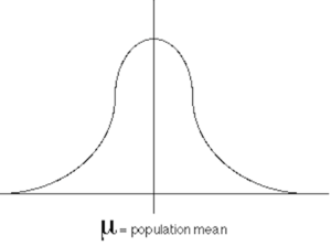
Above is an illustration of the population distribution. As shown in the illustration below, we draw (select, observe, record) the sample distribution from the population distribution.
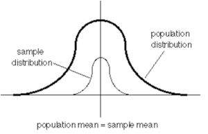
Under the null hypothesis, we test if the mean of the sample is truly representative of the mean for a population. This test is based on the null hypothesis question expressed here: ![]()
Considering an approach in which we use randomized representative sampling to collect our data, we should expect that the sample mean should be the same as the population mean. If this outcome were observed, then we would accept the null hypothesis.
To evaluate the null hypothesis, which is to say, to determine if, in fact, the null hypothesis is true: that the sample represents the population; we compare the sample mean to the population mean, whereby our sample mean is the mean for the set of observations and the population mean is the mean for the set of expected scores.
Therefore, to evaluate the difference between a sample mean and an expected mean we use the Student’s t-test, as shown in the following formula.
[latex]\textit{Student's t-test} = {\overline{x}_{observed}-\overline{x}_{expected}\over{\frac{S_{observed}}{\sqrt{n_{observed}}}}}[/latex]
SAMPLE CALCULATION 29.1
In this first example, we will use the student’s t-test to evaluate the mean score for a continuous random variable for a selection of individuals drawn from a population. In Table 29.1, data for the number of hours in a given month that individuals waited to see their healthcare provider are presented. You are asked to compute the average wait time for this sample and determine if the average for the sample is significantly different than that which is expected in the population.
Table 29.1 Monthly wait time in hours for a random sample of individuals
| Patient ID | Hours Waited |
| 01 | 12 |
| 02 | 13.5 |
| 03 | 8.5 |
| 04 | 4.5 |
| 05 | 10.5 |
| 06 | 15.5 |
| 07 | 12.5 |
| 08 | 9.5 |
| 09 | 11 |
| 10 | 7.5 |
Here we use the Student’s t-test to evaluate the null hypothesis that the observed mean is equal to the expected mean in this set of scores. In the application of the t-test, we assume that the mean score for the sample is representative of the mean score for population, and likewise, that the variance for this sample of scores is an estimate of the variance for the population. We also assume, unless we have some other information, that these data were drawn from a normal distribution.
In this example, we are assessing the null hypothesis: H0: [latex]\overline{x} = \mu[/latex], also presented as H0: [latex]\overline{x} = 0[/latex]. In using the t-test we assume that the population mean [latex][\mu][/latex]has a value of 0 and a variance (standard deviation) of 1. When we are applying the t-test, we are comparing our observed sample mean against the expected population mean of 0 with a variance of 1. The SAS code below produces a test of the null hypothesis using the Student’s t-test.
SAS Code to Compute the Student’s t-Test for a Single Sample
INPUT ID SCORE @@;
DATALINES;
001 12.0 002 13.5 003 08.5 004 04.5 005 10.5 006 15.5 007 12.5 008 09.5 009 11.0 010 07.5
;
PROC SORT DATA=STUDENT; BY ID;
TITLE “STUDENT’S t-TEST TO EVALUATE WAIT TIMES”;
PROC UNIVARIATE; VAR SCORE;
PROC MEANS N MEAN MEDIAN T STDERR PRT;
VAR SCORE; RUN;
The SAS code above produces several important output tables to help us explore our dataset and to evaluate the null hypothesis: H0: [latex]\overline{x} = 0[/latex]. In the output shown below, we can review the descriptive statistics for the dependent variable which we labeled SCORE. In this output we see that the mean score for the sample was 10.5 with a standard deviation of ± 3.17.
Table 29.2 SAS Output for Dependent Variable: SCORE
| N | 10 | Sum Weights | 10 |
| Mean | 10.5 | Sum Observations | 105 |
| Std Deviation | 3.1710496 | Variance | 10.0555556 |
| Skewness | -0.3854798 | Kurtosis | 0.23914105 |
| Uncorrected SS | 1193 | Corrected SS | 90.5 |
| Coeff Variation | 30.2004724 | Std Error Mean | 1.00277393 |
Basic Statistical Measures are given here as location — mean, median and mode, and measures of variability — standard deviation, variance, tang and interquartile range.
Table 29.3 Measures of Location and Variability
| Mean | 10.50000 | Std Deviation | 3.17105 |
| Median | 10.75000 | Variance | 10.05556 |
| Mode | . | Range | 11.00000 |
| Interquartile Range | 4.00000 |
The SAS code also produced statistics that help us to determine a decision with regard to accepting or rejecting the null hypothesis. In Table 29.4 below, we see that the Student’s t value is given as 10.47, and the corresponding p-value was Prt > |t| <0.0001. Because the probability value (Prt) associated with the Student’s t score is <0.05 the outcome indicates that the mean value (10.5 ± 3.17) was significantly different than 0, and therefore we would reject the null hypothesis that H0: [latex]\overline{x} = 0[/latex].
Table 29.4 SAS Output for Tests of [latex]\overline{x} = 0[/latex] Tests for Location: Mu=0
| Test | Statistic | p Value | ||
| Student’s t | t | 10.47095 | Pr > |t| | <.0001 |
| Sign | M | 5 | Pr >= |M| | 0.0020 |
| Signed Rank | S | 27.5 | Pr >= |S| | 0.0020 |
SAMPLE COMPUTATION 29.2
So, what if in this specific example we knew that the real population mean wasn’t 0 but that the mean value was actually a specific number that we determined from the literature. Let’s say that the expected mean should be a value of 10 for this sample. In the following example, we can redo the computations of the Student’s t-test and set the population mean to the specific value of 10. In practice, the value against which the mean is compared should be based on theoretical considerations and/or previous research so that for many experiments the outcome range of the dependent variable can be known.
To test the null hypothesis for the one sample scenario that the expected mean = 10, we compare the t-score observed against the t-score critical. The decision rule then becomes: if the t-test score observed is greater than the t-test score critical then we reject the null hypothesis and state that the sample mean is significantly different than the population mean.
Code to Compute Student’s or Single Sample t-test Using Proc t-test and Setting μ =10
DATA STUDENT;
INPUT ID SCORE @@;
DATALINES;
001 12.0 002 13.5 003 08.5 004 04.5 005 10.5 006 15.5 007 12.5 008 09.5 009 11.0 010 07.5
;
PROC SORT DATA=STUDENT; BY ID;
PROC TTEST H0=10;
VAR SCORE;
TITLE1 “t-TEST WHEN EXPECTED MEAN NOT 0”;
TITLE2 “EXPECTED MEAN = 10”;
RUN;
Table 29.5 “t-TEST WHEN EXPECTED MEAN NOT 0” — “EXPECTED MEAN = 10”
| N | Mean | Std Dev | Std Err | Minimum | Maximum |
| 10 | 10.5 | 3.17 | 1.00 | 4.50 | 15.50 |
| Mean | 95% CL Mean |
| 10.5±3.17 | 8.23[latex]\rightarrow[/latex]12.77 |
| DF | t Value | Pr > |t| |
| 9 | 0.50 | 0.6300 |
In the data presented above, the computed mean was 10.5 with a standard deviation of 3.17. This was compared against an expected mean of 10 and thus produced a t-test score, labeled here as t Value, equal to 0.50. The probability associated with this t-test score is given in the table as Pr >|t|, and is equal to 0.6300. Because the p-value is greater than 0.05 we accept the null hypothesis that the observed mean for the sample is not different than the apriori mean we had set at [latex]\overline{x} = 10[/latex].
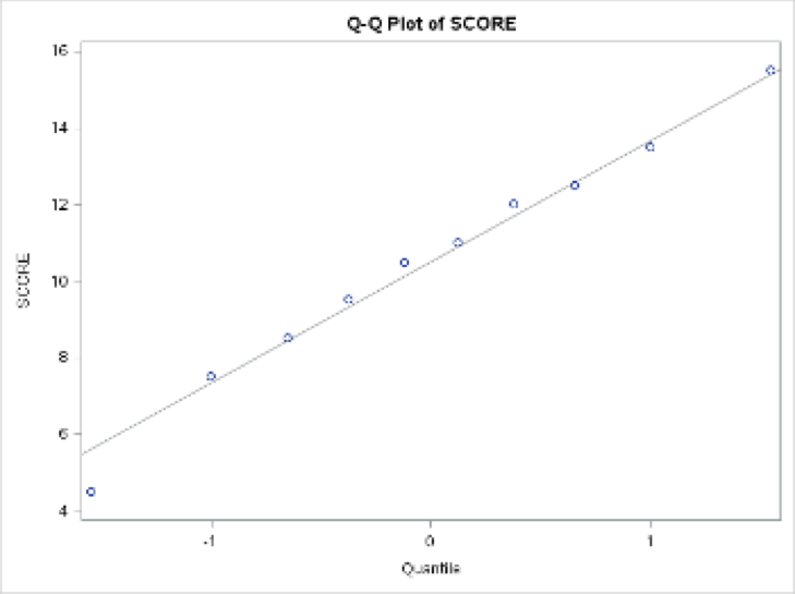
This SAS output for the t-test procedure also produces a Q-Q plot. The Q-Q plot is a visual representation that the data used in this example were drawn from a normal population. If the Q-Q plot presents a relatively straight line then we can assume that the data were drawn from a population that was normally distributed. However, if the data are not representative of a somewhat straight line then we can suggest that the data were not drawn from a population that we would consider to be normally distributed. Notice in Figure 29.1, below, the Q-Q plot shows a straight line and thereby indicates that the data were drawn from a population that was normally distributed.
Figure 29.1 Q-Q plot of data to demonstrate normality in the sample distribution
The Pairwise t-test
To evaluate the significance of the difference in a pre to post design t-test, use the pairwise t-test formula.
Figure 29.2 Evaluating the shift from pretest to posttest
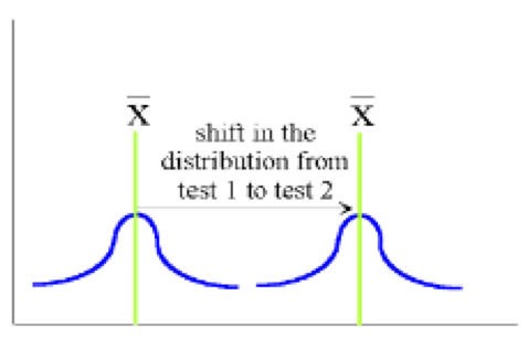
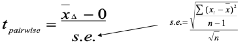
The pre to post (pairwise) t-test measures the amount of shift in the data over the time interval. The formula to compute the pairwise t-test uses the average difference in the measure of interest, from the pre-test score to the post-test score, and then divided by the standard error of the average difference. The standard error of the average difference is computed by dividing the standard deviation of the average difference by the square root of the number of cases in the pairwise comparison.
Figure 29.3 Formula to evaluate the Pre to Post-test design
Computing a Pairwise Comparison T-Test to Evaluate Change
We can use the formula for the pairwise t-test shown above, to compute the significance of the change in the mean score from the pre-test data to the post-test data for the following two sets of 10 numbers.
Pre test data
| Participant Code | 001 | 002 | 003 | 004 | 005 | 006 | 007 | 008 | 009 | 010 |
| Score | 34 | 54 | 60 | 68 | 53 | 70 | 81 | 87 | 65 | 55 |
Post test data
| Participant Code | 001 | 002 | 003 | 004 | 005 | 006 | 007 | 008 | 009 | 010 |
| Score | 44 | 75 | 72 | 98 | 73 | 80 | 91 | 99 | 69 | 76 |
Analyzing these data as a paired t-test.
In this analysis, we will treat the difference scores produced by subtracting the pre-test scores from the post-test scores. In order to do this, we will need to create a new variable. We can create a variable DIFFSCR by subtracting the post-test score from the pre-test scores. As a rule, it is always best to keep our variable names simple and to restrict the label to 8 characters or less. The SAS code to set up this analysis is shown below. However, it is important to note that the degrees of freedom for the paired t-test uses a single sample mean and therefore is df = n – 1, and in this case, df = 10 – 1 = 9 so that the t critical value for α = 0.05 is 2.262 for a two-tailed test and 1.833 for a one-tailed test.
SAS Code to Compute pairwise difference with a t-test
DATA PAIRWISE;
INPUT @1 ID PRETEST POSTTEST;
DIFFSCR=(POSTTEST – PRETEST);
DATALINES;
001 34 44
002 54 75
003 60 72
004 68 98
005 53 73
006 70 80
007 81 91
008 87 99
009 65 69
010 55 76
;
In this analysis, we will evaluate the set of difference scores as a single group (as in a one-sample design) just as we did for the student’s t-test. Under this design, we can use the single-sample t-test or Student’s t-test procedure to compute the significance of the difference scores. Therefore, under this design, we are testing the null hypothesis that the difference between the pre and post scores = 0 (i.e. no difference).
Step 1 in computing the difference scores between the results in the pre test and the results in the post test was to create the variable: DIFFSCR. In this example uses POSTTEST – PRETEST to show a positive change (an increase in score values). The production of the difference score was accomplished with the SAS. command: DIFFSCR=(POSTTEST – PRETEST);
Using the dependent variable DIFFSCR, and the following SAS Code we produced three different SAS outputs: i) PROC UNIVARIATE, ii) PROC MEANS, iii) PROC TTEST.
PROC UNIVARIATE; VAR DIFFSCR;
PROC MEANS N MEAN MEDIAN T STDERR PRT; VAR DIFFSCR;
PROC TTEST; VAR DIFFSCR;
RUN;
The results for each of these procedures are shown below the descriptive statistics produced by the Proc Univariate procedure.
| N | 10 | Sum Weights | 10 |
| Mean | 15 | Sum Observations | 150 |
| Std Deviation | 7.7172246 | Variance | 59.5555556 |
| Skewness | 0.65636272 | Kurtosis | 0.00011636 |
Evaluation of the Null Hypothesis based on output for the UNIVARIATE Procedure
| Test | Statistic | p Value | ||
| Student’s t | t | 6.146532 | Pr > |t| | 0.0002 |
| Sign | M | 5 | Pr >= |M| | 0.0020 |
| Signed Rank | S | 27.5 | Pr >= |S| | 0.0020 |
Evaluation of the Null Hypothesis based on output for the MEANS Procedure
| Analysis Variable: DIFFSCR | |||||
| N | Mean | Median | t Value | Std Error | Pr > |t| |
| 10 | 15.0000000 | 12.0000000 | 6.15 | 2.4404007 | 0.0002 |
Evaluation of the Null Hypothesis based on output for the t-Test Procedure
| DF | t Value | Pr > |t| |
| 9 | 6.15 | 0.0002 |
The important estimates from this output are the mean and variances, which are listed within each of the three SAS procedures. However, each procedure presents the outcome values in different ways. In the PROC UNIVARIATE procedure, all moments of variance are given – standard deviation, variance, skewness, kurtosis, and standard error.
However, in the PROC MEANS procedure only the mean, median, and standard error are reported when the coding above is used. Finally, the PROC TTEST procedure provides the mean score along with the standard deviation and the computation of the confidence limits. In each basic SAS procedure used above, the Student’s t-test computes the comparison between the sample (based on the difference scores) against the population.
Application of the General Decision Rule for the Evaluation of the t-Test
Student’s t-test: H0: sample mean = population mean.
To test this null hypothesis, we compare the t-score observed against the t-score critical. The decision rule is as follows: If the t-score observed is greater than the t-score critical then we reject the null hypothesis and state that the sample mean is significantly different than the population mean.
Pairwise comparisons t-test: H0: mean difference for the sample = mean difference for the population
To test this null hypothesis, we compare the t-score observed against the t-score critical. In this case, the t-score is based on an evaluation of the average difference from pre-test to post-test scores against the expected average difference, in a population of scores, should be 0. The decision rule then becomes: If the t-score observed is greater than the t-score critical then we reject the null hypothesis and state that the change from pre-test scores to post-test scores is significantly different than that which is expected.
t-tests for two independent samples: H0: mean for group1 = mean for group2
Again, to test this null hypothesis we compare the t-score observed against the t-score critical. In this case the t-score is based on a comparison of the difference of the mean for group1 against the mean for group2. The decision rule is as follows: if the t-score observed is greater than the t-score critical then we reject the null hypothesis and state that the two means are significantly different from each other.
Computing a Pairwise Comparison t-Test to Evaluate Change in Resting Blood Pressure
The null hypothesis for the paired or pairwise t-test is given below:
H0: µ1 = µ2 or H0: µ1-µ2=0
In this experiment, a group of 10 individuals agreed to participate in a study of blood pressure changes following exposure to halogen lighting. Resting systolic blood pressure was recorded for each individual. The participants were then exposed to 20 minutes of halogen lighting by playing a video game in a room, which was lit only by halogen lamps. A post-exposure systolic blood pressure reading was recorded for each individual. The results are presented in the following data set.
| ID | 01 | 02 | 03 | 04 | 05 | 06 | 07 | 08 | 09 | 10 |
| SEX | M | F | M | F | M | F | M | F | M | F |
| Pre exposure Systolic BP | 120 | 132 | 120 | 110 | 115 | 128 | 120 | 112 | 110 | 100 |
| Post exposure Systolic BP | 140 | 156 | 145 | 130 | 117 | 148 | 137 | 119 | 127 | 135 |
In the following worksheet we compute the significance of the difference between the pre test blood pressures and the post-test blood pressures..
The null hypothesis is: Ho: µ1 = µ2 and the computation of the variance is shown with the raw data in the table below.
| ID | 01 | 02 | 03 | 04 | 05 | 06 | 07 | 08 | 09 | 10 |
| SEX | M | F | M | F | M | F | M | F | M | F |
| Pre exposure Systolic BP | 120 | 132 | 120 | 110 | 115 | 128 | 120 | 112 | 110 | 100 |
| Post exposure Systolic BP | 140 | 156 | 145 | 130 | 117 | 148 | 137 | 119 | 127 | 135 |
In the following worksheet, we compute the significance of the difference between the pre-test blood pressures and the post-test blood pressures.
The null hypothesis is: Ho: µ1 = µ2 and the computation of the variance is shown with the raw data in the table below.
| ID | sex | pretest BP | post-test bp | pre-post difference [latex]\Delta(x_{i})[/latex] |
| 01 | m | 120 | 140 | 20 |
| 02 | f | 132 | 156 | 24 |
| 03 | m | 120 | 145 | 25 |
| 04 | f | 110 | 130 | 20 |
| 05 | m | 115 | 117 | 2 |
| 06 | m | 128 | 148 | 20 |
| 07 | f | 120 | 137 | 17 |
| 08 | m | 112 | 119 | 7 |
| 09 | f | 110 | 127 | 17 |
| 10 | m | 100 | 135 | 35 |
| [latex]\overline{\Delta}=\sum{\Delta(x_{i})}[/latex] |
| Sum of differences = [latex]\sum \left(\Delta(x_{i}) - \overline{\Delta}\right)[/latex] = 0 | Sum of squared difference scores = [latex]\sum \left(\Delta(x_{i}) - {(\overline{\Delta})}\right)^2[/latex] = 760.1 | |
| [latex]\Delta(x_{i}) - \overline{\Delta}[/latex] | [latex]\left(\Delta(x_{i}) - {(\overline{\Delta})}\right)^2[/latex] | Squared difference scores |
| 20-18.7=1.3 | [latex](1.3)^2[/latex] | 1.69 |
| 24-18.7=5.3 | [latex](5.3)^2[/latex] | 28.09 |
| 25-18.7=6.3 | [latex](6.3)^2[/latex] | 39.69 |
| 20-18.7=1.3 | [latex](1.3)^2[/latex] | 1.69 |
| 2-18.7=-16.7 | [latex](-16.7)^2[/latex] | 278.89 |
| 20-18.7=1.3 | [latex](1.3)^2[/latex] | 1.69 |
| 17-18.7=-1.7 | [latex](-1.7)^2[/latex] | 2.89 |
| 7-18.7=-11.7 | [latex](-11.7)^2[/latex] | 136.89 |
| 20-18.7=-1.7 | [latex](-1.7)^2[/latex] | 2.89 |
| 35-18.7=16.3 | [latex](16.3)^2[/latex] | 265.69 |
To compute the variance for the set of difference scores we divide the sum of squares by n-1. In this analysis the variance is computed as follows.
Sum of squares = [latex]\sum \left(\Delta(x_{i}) - {(\overline{\Delta})}\right)^2 = {760.1 \over{n - 1}} = {760.1 \over{10-1}} = {760.1 \over{9}} = 84.46[/latex]
The standard deviation is then calculated by estimating the square root of the variance. Here the calculation is the square root of 84.46, which produces a standard deviation of 9.19. Once we have the standard deviation we can calculate the standard error by dividing the standard deviation by the square root of n. Here we have a standard deviation of 9.19 and n=10 (our total sample). The calculation of the standard error is then 9.19 divided by the square root of 10 which equals 2.91, as shown below.
[latex]s = \sqrt{84.46} = 9.19 [/latex] [latex]\textit{s.e.} = {s\over\sqrt{n}}[/latex] [latex]\rightarrow \textit{s.e.} = {9.19\over\sqrt{10}} = 2.91[/latex]
Once we have the standard error from these calculations then we can calculate the t-test value. Recall that the t-test score provides an evaluation of the null hypothesis which here is a test that the mean difference between the pre and post blood pressure scores is equal to 0. The calculation for the t score in this scenario is shown here:
[latex]t = \left( \overline{\Delta} - 0 \over{s.e.}\right)[/latex] [latex]\rightarrow t = \left(18.7 - 0 \over{2.91}\right)[/latex] [latex]\rightarrow t = \left(6.43\right)[/latex]
Next use the t observed score to evaluate the null hypothesis by comparing the t observed scores against the t expected score for a research design in which we started with a sample of n=10. The t expected score is identified in a table of critical values — easily retrieved from the internet. The information required to identify the t critical value is the number of cases in our sample and the probability level at which we want to be sure that we are making the right decision in regard to accepting or rejecting the null hypothesis. For most research studies we accept that we want to be 95% confident that we are making the correct decision in regard to accepting or rejecting the null hypothesis, so given that (100% – 95% = 5%) we establish a probability level of 0.05 or 5%; and we call this probability the alpha level. Once we have our alpha level and we know our sample size (n) then we can look up the appropriate t critical value (from a standard table of critical values) against which we will compare our t observed score.
In the evaluation of changes in blood pressure, our t observed score was 6.43, and the corresponding t critical (or t expected) score based on an alpha level of 0.05 and n=10 is given as t critical = 2.228. Therefore, since our t observed score (tobserved = 6.43) is greater than the t critical score (tcritical = 2.228) we reject the null hypothesis [latex]H_{0}: \left( \overline{\Delta} = 0 \right)[/latex] and determine that the change in blood pressures within our sample was statistically significant.
In this analysis, we can write a SAS program to evaluate the pairwise t-test using the PROC MEANS procedure and evaluate the null hypothesis using both Proc MEANS, as well as the student’s single sample t-test. The SAS program is as follows:
DATA PAIRWISE;
INPUT @1 ID SEX $ PREBP POSTBP;
Following the input paragraph above, we create a new variable to represent the difference in pre to post systolic blood pressure scores. Here we will call this variable DELTABP. Considering that post bp is expected to rise following exposure to halogen, we include POSTBP as the first term in the equation to compute the difference scores.
DELTABP = (POSTBP – PREBP);
DATALINES;
01 m 120 140
02 f 132 156
03 m 120 145
04 f 110 130
05 m 115 117
06 m 128 148
07 f 120 137
08 m 112 119
09 f 110 127
10 m 100 135
;
Computing the pairwise t-test is similar to computing the student’s or single sample t-test. Here we use the measure of difference scores as the variable of interest. The SAS procedural commands are presented here:
PROC SORT DATA=PAIRWISE; BY ID;
PROC UNIVARIATE; VAR DELTABP; RUN;
In the statement below, we use PROC MEANS to compute the t-test scores. Notice that the options to produce the statistical output are included within the PROC MEANS statement prior to the semi-colon.
PROC MEANS N MEAN MEDIAN T STDERR PRT; VAR DELTABP; RUN;
In the statement below, we use PROC TTEST to compute the t-test scores.
PROC TTEST; VAR DELTABP; RUN;
As in all analyses we begin with the descriptive statistics. These are reported through the output for the PROC UNIVARIATE procedures. However, since we are comparing a mean for a sample against the population mean of 0, we really don’t need to do much more as SAS provides this outcome in the reporting of the student’s t-test as part of the PROC UNIVARIATE procedure, shown below.
Table 29.6. Output from PROC UNIVARIATE for dependent variable: DELTABP
| N | 10 | Sum Weights | 10 |
| Mean | 18.7 | Sum Observations | 187 |
| Std Deviation | 9.18997038 | Variance | 84.4555556 |
| Skewness | -0.2742618 | Kurtosis | 0.84720499 |
| Coeff Variation | 49.1442266 | Std Error Mean | 2.9061238 |
| Test | Statistic | p Value | ||
| Student’s t | t | 6.43 | Pr > |t| | 0.0001 |
| Sign | M | 5 | Pr >= |M| | 0.0020 |
| Signed Rank | S | 27.5 | Pr >= |S| | 0.0020 |
Next, the PROC MEANS procedure was used to compute the mean and test the comparison of the mean from 0 using the single sample t-test. The output is shown below. Notice this procedure lists the t-value and the probability of the computed t-value.
Table 29.7. Output from PROC MEANS for dependent variable: DELTABP
| N | Mean | Median | t Value | Std Error | Pr > |t| |
| 10 | 18.7000000 | 20.0000000 | 6.43 | 2.9061238 | 0.0001 |
The values computed with the PROC MEANS procedure can be compared to the procedures of the PROC TTEST and are shown below for the pairwise t-test comparison.
Table 29.8. Output from PROC TTEST for dependent variable: DELTABP
| N | Mean | Std Dev | Std Err | Minimum | Maximum |
| 10 | 18.7000 | 9.1900 | 2.9061 | 2.0000 | 35.0000 |
| Mean | 95% CL Mean | |
| 18.7000 | 12.1259 | 25.2741 |
Again, the important bits of information are the t-value and the probability of the t-value. The evaluation of the t-value is to consider the likelihood of the computed value. Recall that there is no fixed demarcation point for this t-test outcome, but what is more important is whether the differences are as expected. Using a probability estimate of p<0.05 as a guide we can decide about the difference in means relative to the t-test score. Here we see that the t-test score is 6.43 and the associated probability of observing this t-test value is less than 0.05.
| DF | t Value | Pr > |t| |
| 9 | 6.43 | 0.0001 |
However, what we really want to talk about is what this difference means to your research question. In this instance, the results indicate that the mean systolic blood pressure, measured prior to exposure to the halogen lights was significantly lower than the mean systolic blood pressure, measured after exposure to the halogen lights.
Notice, also that the values computed with the SAS program for each of the procedures verify the calculations that we worked through by hand, above. That is: the mean difference score was 18.7 with a variance estimate of 84.45, a standard deviation of 9.19, a standard error score of 2.906 (rounded to 2.91) and a t-test score of 6.43. Well done, SAS!
