
Parametric Statistics
26 Measures of Central Tendency
PART 1: Measures of Central Tendency
The most common measure of central tendency is the mean or average score. The mean is a calculated score that is intended to represent all of the scores in the distribution (set of scores).
The formula for the mean of a sample is shown here:
[latex]{\overline{x}} = \Sigma{(x_i)\over{n}}[/latex]
Where:
- [latex]{\overline{x}}[/latex] refers to the sample mean
- [latex]\Sigma{(x_i)} refers to the sum of all the scores
- i refers to the “ith” case within the distribution
- n refers to all of the cases within the distribution.
To calculate the mean for a continuous variable, add up all of the values and divide the sum of values by the number of values. Below is a set of blood glucose measures for 5 patients. These data are represented in millimoles per litre (mmol/L). Pn represents the nominal value label for each patient, so that P1 is patient 1. P1 4.2 mmol/L, P2 5.6 mmol/L, P3 7.9 mmol/L, P4 10.2 mmol/L, P5 7.5 mmol/L, Follow these steps to calculate the mean:
- First add the values together: 4.2 + 5.6 + 7.9 + 10.2 + 7.5 = 35.4.
- Next, divide by the number of values (to produce the average): 35.4/5 = 7.08 mmol/L
We can also use SAS to compute the mean for a set of scores. Two specific SAS programs that process measures of central tendency are PROC MEANS, and PROC UNIVARIATE. Each of these programs was designed to produce descriptive statistics for a sample of scores. Below are the SAS commands to compute the mean for a set of 10 resting heart rate scores. In this first program we used the SAS procedural command PROC MEANS to compute three basic estimates: the mean, the standard deviation and the minimum/maximum scores for the sample dataset of 10 numbers.
Notice in the code written above, the semi-colon (;) is placed on a separate line below the set of scores. While PROC MEANS, in its simplest form (without options) provides three basic estimates that describe estimates within a distribution, the SAS procedural command PROC UNIVARIATE not only computes the mean but also creates the Basic Statistical Measures Table which provides an entire summary of descriptive statistics. The output generated by the SAS program above – using the PROC MEANS statement without options – produced a table of summary estimates that included the mean and standard deviation as well as the minimum and maximum values for the dataset. SAS Output from the MEANS Procedure: Variable of interest was Heart Rate
| N | Mean | Std Dev | Minimum | Maximum |
| 10 | 61.80 | 11.56 | 48.00 | 84.00 |
When we call the PROC UNIVARIATE procedure of SAS, the output is a more complete table of summaries that include estimates of centrality but also the moments, measures of variance, and the tests of the location of the mean, as shown below.
SAS PROC UNIVARIATE to Produce Descriptive Statistics for a Sample of 10 Numbers
The UNIVARIATE Procedure -- Variable: SCORE
| MOMENTS | |||
| N | 10 | Sum Weights | 10 |
| Mean | 61.8 | Sum Observations | 618 |
| Std Deviation | 11.5547008 | Variance | 133.511111 |
| Skewness | 0.55954538 | Kurtosis | -0.2284272 |
| Uncorrected SS | 39394 | Corrected SS | 1201.6 |
| Coeff Variation | 18.6969269 | Std Error Mean | 3.65391723 |
| Tests for Location: Mu0=0 | ||||
| Test | STATISTIC | ESTIMATE | p Value | |
| Student's t | t | 16.91336 | Pr > |t| | .0001 |
| Sign | M | 5 | Pr >= |M| | 0.0020 |
| Signed Rank | S | 27.5 | Pr >= |S| | 0.0020 |
Comparing the Mean for a Sample to the Expected Mean for a Population
In the output from the PROC UNIVARIATE procedure, SAS includes a table in which the mean for the variable: SCORE is compared to the mean for the Standard Normal Distribution (SND). The SND represents the hypothetical population mean and has a value of 0 with a standard deviation of 1. In the SAS table shown above, entitled Tests for Location: Mu0=0 the comparison of the sample mean ([latex]{\overline{x}}[/latex] ) to the population ([latex]{\mu}[/latex] ) is evaluated with the Student’s t-Test.
The results presented in the table above show that the Student’s t-Statistic value is 16.91 and the probability associated with this estimate is <0.001. Together these values indicate that the observed sample mean is significantly different than the hypothesized expected mean for the population (set at Mu0=0) from which the sample was drawn.
However, what if we wanted to establish a suggested value for the population mean that is not 0, but that is based on value reported in the literature? In this case, we could assign a suggested value to the population mean and then compare the observed mean for the sample to the expected value for a population. In the following code, we test this notion.
Assign a suggested value to the population mean
PROC TTEST H0=54
PLOTS(SHOWH0)
ALPHA=0.05;
VAR SCORE;
RUN;
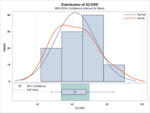
The SAS output is given below. The results indicate that the average score for the sample ([latex]{\overline{x}}[/latex] = 61.80) is not significantly different at the probability level of p < 0.05 than the expected score of ([latex]{\mu}[/latex] =54). Notice, in addition to the table of output SAS also includes a graph illustrating the shape of the distribution and the comparison of the sample estimate to the expected population estimate of centrality.
| The t-test Procedure | ||
| DF | t Value | Pr > |t| |
| 9 | 2.13 | 0.0615 |
| Parameter estimates | ||
| Mean | 95% CL Mean | |
| 61.8000 | Lower limit: 53.5343 | Upper Limit: 70.0657 |
Considering that the confidence interval shown here includes the mean for the sample (61.8) and the mean for the population which we set apriori as 54, no significant difference is observed, between that which is expected and that which was observed. This estimate is illustrated in the following graph.
Calculate the Mean for A Frequency Distribution
In the following example, we compute the mean for frequency distribution. The formula to compute the mean of a frequency distribution is shown here as:
[latex]{\overline{x}} = {\Sigma{fx_i}\over{n}}[/latex]
Where:
- f refers to the frequency in each interval
- xi refers to the mid-point of the interval
- i refers to the “ith” case within the distribution
- n refers to all of the cases within the distribution.
Below is the frequency distribution table for the heights of 200 individuals. The data represent heights recorded in centimetres and organized into seven categories. The SAS code to compute the mean for this set of data is shown below the table. Notice that the table is reduced to a simple composition of two variables which includes the mid-point of the category represented by the variable: GRPMDPT, and the number of individuals, whose height scores fall within the specific category, represented by the variable: COUNTS.
| Column 1
cell boundaries |
Column 2 frequency (f) | Column 3
cell mid-point |
Column 4
(f) x cell midpoint |
Column 5
(col 4 ÷ n) |
| 158.5 – 161.5 | 4 | 160 | 4 x 160 = 640 | 640/200 = 3.2 |
| 161.5 – 164.5 | 12 | 163 | 12 x 163 = 1956 | 1956/200 = 9.78 |
| 164.5 – 167.5 | 44 | 166 | 44 x 166 = 7304 | 7304/200 = 36.52 |
| 167.5 – 170.5 | 64 | 169 | 64 x 169 = 10816 | 10816/200 = 54.08 |
| 170.5 – 173.5 | 56 | 172 | 56 x 172 = 9632 | 9632/200 = 48.16 |
| 173.5 – 176.5 | 16 | 175 | 16 x 175 = 2800 | 2800/200 = 14.00 |
| 176.5 – 179.5 | 4 | 178 | 4 x 178 = 712 | 712/200 = 3.56 |
| [latex]{\overline{x}} = {\Sigma{fx_i}\over{n}}[/latex] | [latex]{\overline{x}} = {33860\over 200}[/latex] | = 169.3 | The [latex]{\overline{x}}[/latex] is the sum of column 5 |
The SAS code to compute the mean for data in the table above
DATA FREQMN;
INPUT GRPMDPT COUNTS @@;
CRSPRDCT= GRPMDPT*COUNTS;
/* COMPUTE RATIO FOR THE CROSS PRODUCT USING GROUP MIDPOINT X CELL FREQUENCY */
XP_RATIO=CRSPRDCT/200;
LABEL GRPMDPT = ‘GROUP MIDPOINT’
COUNTS = ‘NUMBER OF CASES PER CELL’
CRSPRDCT = ‘CROSS PRODUCT PER CELL’
XP_RATIO = 'CROSS PRODUCT RATIO';
DATALINES;
160 4 163 12 166 44 169 64 172 56 175 16 178 4
;
PROC PRINT;
VAR GRPMDPT COUNTS CRSPRDCT XP_RATIO;
SUM CRSPRDCT XP_RATIO;
FOOTNOTE1 "* THE MEAN IS PRODUCED AS THE SUM OF THE VARIABLE XP_RATIO";
FOOTNOTE2 "** THE MEAN CAN ALSO BE CALCULATED FROM THE SUM OF THE VARIABLE CRSPRDCT ÷ 200";
RUN;
The output generated by the SAS program above is the table of raw data presented in column form and includes the sums of the columns used to compute the mean for the frequency distribution.
| Obs | grpmdpt | counts | crsprdct | cp_ratio |
| 1 | 160 | 4 | 640 | 3.20 |
| 2 | 163 | 12 | 1956 | 9.78 |
| 3 | 166 | 44 | 7304 | 36.52 |
| 4 | 169 | 64 | 10816 | 54.08 |
| 5 | 172 | 56 | 9632 | 48.16 |
| 6 | 175 | 16 | 2800 | 14.00 |
| 7 | 178 | 4 | 712 | 3.56 |
| 33860 | 169.30 |
* The mean is produced as the sum of the variable XP_RATIO
** The mean can also be calculated from the sum of the variable crsprdct ÷ 200
The Weighted Mean Score
In some situations, we may wish to combine means from several samples. Under such circumstances, we need to consider the sample size (or weight) of the distribution from which the means were drawn. By adjusting each independent sample mean by the number of subjects in the respective sample from which the means were drawn, we are able to provide different relative contributions of each mean to the total mean of all samples combined. The formula for a weighted mean from two samples is shown here. The formula for the mean of a sample is shown here:
[latex]{\overline{x}}={n_i\times{\overline{x_1}}+n_2{\overline{x_2}}\over{n_1 + n_2}}[/latex]
The Median Score
The median score is also a measure of central tendency, and it is defined as the middle score in a set of ordered scores. In the example below, we begin with a set of scores (an array), we next sort the scores from lowest to highest. Then we identify the number that is in the middle of the ordered set of scores where half the numbers are above the identified middle score, and half the numbers are below the identified middle score.
Example: Median
The median is the middle score. Considering the heart rate values again, we put these readings in order of magnitude and then identify which value is in the middle:
- 57
- 59
- 59
- 75
- 78
- 78
- 85
- 88
- 88
- 88
In this case, we have an even number of values (n = 10) so we can calculate the average of the two values in the middle. It just so happens that they are the same value in this example (78) so the median is 78.
- initial array of scores: {12, 72, 56, 34, 35, 13, 36, 16, 67}
- sorted array of scores: {12, 13, 16, 34, 35, 36, 56, 67, 72}
- sorted array of scores: {12, 13, 16, 34, 35, 36, 56, 67, 72}
Notice in the example above, regardless of the actual scores, the middle score in the ordered set of scores is the median, which in this set is 35.
When we have an even number of scores in our array there is a special caveat to identifying the median score in the distribution (set of scores). When we have two scores selected as the identified middle score we simply compute the average between the two identified middle scores and use that number as the median score. That is, we add the two middle scores together and divide by 2.
- initial array of scores: {22, 32, 86, 44, 25, 13, 16, 18, 47, 11}
- sorted array of scores: {11, 13, 16, 18, 22, 25, 32, 44, 47, 86}
- computed median for the array: {11, 13, 16, 18, 22, 23.5, 25, 32, 44, 47, 86}
The Mode Score
The mode score is the third measure of central tendency, and it is defined as the most frequently occurring score in a set of scores. In the example below, we simply count the number of scores that are the same within a set of scores, within an array or within a distribution.
Below are 10 resting heart rate values:
78, 88, 57, 59, 75, 85, 88, 78, 59, 88
The mode is 88 because it appears most often.
In the following example of 16 scores, the number 2 occurs 3 times, but the number 27 occurs 4 times therefore we would identify 27 as the mode score.
2, 2, 2, 5, 6, 14, 15, 23, 26, 27, 27, 27, 27, 28, 37, 41
