
Analysis of Non-Parametric Outcomes
24 Computing the Wilcoxon-Mann-Whitney U Test
The Wilcoxon Mann-Whitney is a 2 group non-parametric comparison test equivalent to the Parametric t-test that can be used to test treatment effects when data are not normally distributed.
- The Mann-Whitney U test, which may also be referred to as the Wilcoxon-Mann-Whitney test, or the Wilcoxon Rank-Sum test, evaluates the ranks of the combined scores from two independent groups.
- The Wilcoxon rank-sum test statistic (referred to as Ws if using the name Wilcoxon rank-sum) is based on using the sum of the ranks for observations drawn from one of the groups within the sample of data.
Generally, the groups being studied are designated as GROUP 1 = treatment group and GROUP 2 = control group. This statistic — regardless of whether you refer to it as the Mann-Whitney test or the Wilcoxon rank-sum test, is considered to be among the more powerful of the non-parametric statistical procedures; and when using large samples, the computational result of this test is generally the same as the parametric t-test for two independent groups.
When evaluating the outcome of this statistic, we can test the Wilcoxon rank-sum test statistic against a critical value from a table of standard values, or we can compute a z-score for the comparison of ranks.
In the Mann-Whitney U— Wilcoxon rank-sum test we compute a “z score” (and the corresponding probability of the “z score”) for the sum of the ranks within either the treatment or the control group. The “U” value in this z formula is the sum of the ranks of the “group of interest” – typically the “treatment group”.
Essential Formulae
Below is the formula to compute z score for the Wilcoxon-Mann-Whitney test:
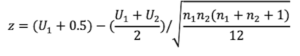
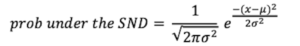
The formula to compute the probability of arriving at the z that you computed under the standard normal distribution (SND) is shown in this next formula. We use this probability value to evaluate the outcome of the Mann-Whitney test. In this formula, replace the x term with z from the formula above. The value for π is 3.14, the value for σ2 is 1, the value for μ is 0.
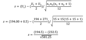
A working example:
You conducted a study to determine if a new treatment procedure was better than the standard method. 30 participants were recruited from a population of students and randomly allocated to either the new treatment procedure (T) or the standard method (S) so that the initial distribution was set at (n1 = 15 and n2 = 15).
After applying the treatments to each group respectively the students were ranked on a specific measure that demonstrates the influence of the two treatment methods. The ranks for each response score are given in the following table while maintaining the student’s group membership.
NT= New treatment; ST = Standard Treatment
| Row 1: Participant ID | 1 | 2 | 3 | 4 | 5 | 6 | 7 | 8 | 9 | 10 | 11 | 12 | 13 | 14 | 15 |
| Row 2: Dependent Variable Scores | 8 | 12 | 13 | 15 | 19 | 21 | 22 | 28 | 31 | 36 | 37 | 39 | 40 | 41 | 43 |
| Row 3: Group codes | NT | NT | NT | ST | ST | NT | NT | ST | ST | ST | NT | NT | NT | NT | NT |
| Row 4: Rank of score | 1 | 2 | 3 | 4 | 5 | 6 | 7 | 8 | 9 | 10 | 11 | 12 | 13 | 14 | 15 |
| Row 1: Participant ID | 16 | 17 | 18 | 19 | 20 | 21 | 22 | 23 | 24 | 25 | 26 | 27 | 28 | 29 | 30 |
| Row 2: Dependent Variable Scores | 48 | 52 | 53 | 55 | 59 | 61 | 62 | 68 | 71 | 76 | 77 | 79 | 80 | 81 | 83 |
| Row 3: Group codes | NT | NT | NT | ST | ST | ST | ST | ST | ST | ST | ST | ST | ST | NT | NT |
| Row 4: Rank of score | 16 | 17 | 18 | 19 | 20 | 21 | 22 | 23 | 24 | 25 | 26 | 27 | 28 | 29 | 30 |
Values in Row 2 in the table above represent the score on the dependent variable measuring the response to the two treatment types.
Values in Row 3 in the table above represent the codes for the group membership, where T=new treatment method group and S=standard method group.
Values in Row 3 in the table above represent the Rn= rank of participants within the total data set.
Ranks begin from the lowest score to the highest score.
The sum of the ranks (U1) in the NEW Treatment group are: (1+2+3+6+7+11+12+13+14+15+16+17+18+29+30) = 194
The sum of the ranks (U2) in the STANDARD Treatment group are: (4+5+8+9+10+19+20+21+22+23+24+25+26+27+28) = 271
What about ties?
In the case of a tie, we simply organize all of the data as in the table above, and then we assign each observation in a tie its average rank. So if we had two scores 12 and 12 and they had a rank of 3 and 4 then we would simply give the first value of 12 a rank of 3.5 and the second value of 12 a rank of 3.5.
Verifying the Computations with SAS
DATA MWW;
INPUT ID GROUP SCORE @@;
CARDS;
01 1 8 02 1 12 03 1 13 04 2 15 05 2 19 06 1 21 07 1 22 08 2 28 09 2 31
10 2 36 11 1 37 12 1 39 13 1 40 14 1 41 15 1 43 16 1 48 17 1 52 18 1 53
19 2 55 20 2 59 21 2 61 22 2 62 23 2 68 24 2 71 25 2 76 26 2 77 27 2 79
28 2 80 29 1 81 30 1 83
;
PROC PRINT; VAR ID GROUP SCORE;
PROC NPAR1WAY DATA=MWW WILCOXON;
CLASS GROUP; VAR SCORE; EXACT;
RUN;
The NPAR1WAY PROCEDURE OUTPUT
Wilcoxon Scores (Rank Sums) for Variable score: Classified by Variable group
| GROUP | N | Sum of Scores |
Expected Under H0 |
Std Dev Under H0 |
Mean Score |
| New Treatment | 15 | 194.0 | 232.50 | 24.109127 | 12.933333 |
| Standard Treatment | 15 | 271.0 | 232.50 | 24.109127 | 18.066667 |
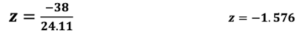
Wilcoxon Two-Sample Test: Z includes a continuity correction of 0.5 –> Statistic (S) = 194.00
Normal Approximation: Z = -1.5762; One-Sided Pr < Z = 0.0575; Two-Sided Pr > |Z| = 0.1150. EXACT TEST: One-Sided Pr <= S = 0.0580; Two-Sided Pr >= |S – Mean| = 0.1160.
Your Turn
Compute the Sign Test and the Mann-Whitney Test
You are interested in the effects of daily exercise on fitness levels.
You create an experiment in which individuals are allocated to either a twelve-week exercise program or a sedentary control group. You were successful in recruiting 30 subjects, and you matched these individuals on gender and exercise profiles to balance the groups that will either participate or remain sedentary.
You arrange the participants into two groups (n1=15, and n2=15). Group 1 receives a 12-week regimen of noon-hour exercises while Group 2 is considered the control group and does not receive any exercise programming or any related information. Both groups maintain very nearly similar profiles for sleep and diet. The probability of being selected as an exerciser is 50% or “p= ½”, and conversely the probability of being selected to the control group is 50% or “p= ½”
The dependent variable for the experiment is the measure of the individual’s predicted VO2 max as determined by a sub-maximal walking test. Given this scenario and research design, you decide to use the “SIGN TEST” as the statistical procedure to determine if the exercise regimen caused significant changes in the fitness levels of the participants compared to the control group members. The data for this experiment are presented in DATA SET #1 below. COMPLETE THE TABLE, and compute the significance of the sign test.
Data Set #1 – Computing the significance of the Z statistic in the “Sign test”
| VO2 Grp1 (ml/ kg·min-1) |
VO2 Grp2 (ml/ kg·min-1) |
Comparison of VO2 max test scores |
Sign of |
| 43 | 40 | Subject1Group1 > Subject1Group2 | + |
| 48 | 42 | Subject2Group1 Subject2Group2 | |
| 39.4 | 43.8 | Subject3Group1 < Subject3Group2 | – |
| 32.7 | 31.9 | Subject4Group1 > Subject4Group2 | |
| 36.9 | 48.4 | Subject5Group1 Subject5Group2 | |
| 50.2 | 41.4 | Subject6Group1 Subject6Group2 | + |
| 39.9 | 31.9 | Subject7Group1 Subject7Group2 | |
| 45.3 | 33.2 | Subject8Group1 Subject8Group2 | |
| 40.8 | 39.6 | Subject9Group1 Subject9Group2 | |
| 39.8 | 41.2 | Subject10Group1 Subject10Group2 | |
| 45.4 | 43.5 | Subject11Group1 > Subject11Group2 | |
| 57.3 | 52.5 | Subject12Group1 Subject12Group2 | + |
| 58.7 | 40.6 | Subject13Group1 Subject13Group2 | |
| 35.4 | 39.5 | Subject14Group1 Subject14Group2 | |
| 58.4 | 49.5 | Subject15Group1 > Subject15Group2 | + |
Null hypothesis |
Number of (+) or (-) SIGNS |
Z sign test |
The decision concerning the null hypothesis |
Recall that in our study we had N = 30 where we created two matched groups of 15 subjects per group. Treatment group is GROUP 1 and Control group is GROUP 2.
As a follow-up to the study, you decided to compare average resting heart rate responses for the group of individuals who participated in the “lunch-hour exercise group”, against the sedentary control group, over the twelve-week timeline.
The data for this study are presented in Data Set #2 below. Given the arrangement of data, recall that you are attempting to measure if the heart rates for the “lunch-hour exercise group” are generally higher or lower than the heart rates for the sedentary control group. Since you expect that twelve weeks of exercise at lunch hour should have a positive effect on the cardiovascular system, you also expect that the resting heart rates for the “lunch-hour exercise group” would be generally lower than the heart rates for the sedentary control group.
Use the Mann-Whitney test to compute a “z score” for the sum of the ranks within either the treatment or the control group. Include the null hypothesis and your decision about the null hypothesis based on the computations.
Data Set #2 – Computing the Mann Whitney Statistic
n1 (the exercise group) = 11 (use EG as the exercising group code).
EG = 89, 95, 103, 105, 109, 113, 114, 115, 117, 123, 128
n2 (the sedentary control group) = 9 (use CG as the control group code)
CG = 100, 101, 107, 119, 126, 134, 135, 136, 139
ROW 1: Scores arranged from lowest to highest
ROW 2: Group membership for scores (E= experimental, C= control)
ROW 3: Rank position for scores (beginning lowest score to highest)
| ROW 1 | 89 | 103 | 113 | 126 | 139 | |||||||||||||||
| ROW 2 | E | E | C | E | E | C | C | C | ||||||||||||
| ROW 3 | 1 | 2 | 4 | 5 | 9 | 15 | 19 | 20 |
| Null hypothesis | U1 | Sum of ranks in the control group | Z Mann-Whitney | The decision concerning the null hypothesis |
