
| Statistic | DF | Value | Prob |
|---|---|---|---|
| Chi-Square | 4 | 1.8010 | 0.7723 |
| Likelihood Ratio Chi-Square | 4 | 1.8049 | 0.7716 |
| Mantel-Haenszel Chi-Square | 1 | 0.7697 | 0.3803 |
| Phi Coefficient | 0.1026 | ||
| Contingency Coefficient | 0.1021 | ||
| Cramer’s V | 0.1026 |
Goodness of Fit and Related Chi-Square Tests
17 The Goodness of Fit Test for Two Groups
The Two-Sample Chi-Square Goodness of Fit Test
In this chapter, we will work through examples of the Goodness of Fit chi-square when we have two groups. Here we will use both SAS coding as well as the two sample webulator for a goodness of fit test. The two sample webulator enables us to compare the distribution of responses for one sample against the distribution of the responses for a second sample.
In the following example, we applied the goodness of fit test for a sample of individuals that were asked about their health status. The tool to collect the information was the RAND SF-36. In this example, we also added demographic information to represent sex, and although the response categories for SEX were (1=male, 2=female and 3=other) we processed the data as a binary outcome (males versus females). The data set was comprised of three variables which included id, sex and the individual’s response to the five-item question: 1. In general, would you say your health is: i) Excellent, ii) Very good, iii) Good, iv) Fair, v) Poor.
The relevant SAS code added to process the 2 group chi-square goodness of fit test
PROC FORMAT;
VALUE HEAFMT 1 = EXCELLENT 2 = VERY GOOD 3 = GOOD 4 = FAIR 5 = POOR;
VALUE GENFMT 1=MALE 2=FEMALE 3=OTHER;DATA CHIGF2;
INPUT ID SEX HEALTH @@;LABEL HEALTH=’OPTIONS FOR RAND SF-36 HEALTH QUESTION’;
TITLE ‘TWO GROUP GOODNESS OF FIT FOR HEALTH STATUS RAND SF-36 ‘;DATALINES;
001 1 1 002 1 2 003 1 3 004 1 4 005 1 5 006 2 1 007 2 2 008 2 3 009 2 4 010 2 5 011 3 1 012 1 2 013 3 3 014 1 4 015 1 5 016 2 1 017 2 2 018 2 3 019 2 4 020 2 5 021 1 1 022 1 2 023 1 3 024 1 4 025 1 5 026 2 1 027 2 2 028 2 3 029 2 4 030 2 5 041 1 1 042 1 1 043 1 1 044 1 1 045 3 1 046 2 1 047 2 1 048 2 1 049 2 1 050 3 1 031 1 5 032 1 5 033 1 5 034 3 5 035 1 5 036 2 5 037 3 5 038 3 5 039 2 5 040 2 5 101 1 1 102 1 2 103 1 3 104 1 4 105 1 5 106 2 1 107 2 2 108 2 3 109 2 4 060 3 5 061 3 1 062 1 2 063 1 3 064 1 4 065 1 5 066 2 1 067 3 2 068 2 3 609 2 4 700 3 5 081 1 1 082 3 2 083 1 3 084 1 4 085 1 5 086 3 1 087 2 2 088 2 3 089 2 4 090 2 5 081 1 1 082 1 1 083 1 1 084 1 1 085 1 1 086 2 1 087 2 1 088 2 1 089 2 1 080 2 1 051 3 5 052 3 5 053 1 5 054 1 5 055 1 5 056 2 5 057 3 5 058 3 5 059 2 5 100 2 5 160 2 5 161 3 1 162 1 2 613 1 3 641 1 4 651 1 5 166 2 1 167 3 2 168 2 3 169 2 4 170 2 5 181 1 1 182 1 2 183 3 3 184 1 4 185 3 5 186 2 1 187 2 2 188 2 3 189 3 4 190 2 5 181 3 1 182 1 1 288 3 1 289 2 1 280 2 1 251 1 4 252 1 3 253 1 4 254 3 3 255 1 4 256 2 3 257 2 4 258 2 4 259 2 3 100 2 2 160 2 5 161 1 1 162 1 2 613 1 3 641 1 4 651 1 5 166 2 1 167 2 2 988 2 1 389 2 3 380 2 1 351 3 5 352 1 5 353 1 5 354 1 5 355 1 5 356 2 5 357 3 5 358 2 5 359 2 5 100 2 5 160 2 5 161 1 1 162 3 2 613 1 3 641 1 4 651 1 5 166 2 1 167 2 2 560 2 5 561 1 1 562 1 2 563 1 3 564 1 4 565 1 5 566 2 1 567 2 2 568 2 3 569 2 4 570 2 5 581 1 1 582 1 2 583 1 3 584 3 4 585 1 5 586 2 1 587 2 2 588 2 3 589 2 4 590 3 5 581 1 1 582 1 2 583 1 2 584 1 2 585 1 2 586 3 2 587 2 1 588 2 1 589 2 3 580 3 3 551 1 3 552 1 5 553 1 4 554 1 5 555 1 4 556 3 5 557 2 4 558 2 4 559 3 3
;
/* PRODUCE A HISTOGRAM FOR THE ENTIRE SET OF DATA*/PROC SORT DATA=CHIGF2; BY SEX;
PROC SGPLOT; HISTOGRAM HEALTH;
FORMAT HEALTH HEAFMT. ;
RUN;/* CALCULATE CHI SQUARE GOODNESS OF FIT – MALES VS FEMALES */PROC FREQ;
TABLES HEALTH*SEX/CHISQ;
WHERE SEX<3; /* RESTRICT DATA TO A TWO GROUP COMPARISON */
FORMAT HEALTH HEAFMT. SEX SEXFMT. ;
TITLE ‘FREQUENCY DISTRIBUTION FOR SELF-REPORTED HEALTH STATUS’;
TITLE2 ‘TWO SAMPLE GOODNESS OF FIT STUDY’;
RUN;/*CREATE A GRAPH USING COLORS */
/* Define the axis characteristics */
axis1 offset=(0,70) minor=none;
axis2 label=(angle=90);
pattern1 value=solid color=cx7c95ca;
pattern2 value=solid color=cxde7e6f;proc sort; by SEX;
proc gchart ;
vbar HEALTH / SUBGROUP=SEX TYPE=PERCENT
discrete raxis=axis2;
WHERE SEX<3; /* RESTRICT DATA TO A TWO GROUP COMPARISON */
FORMAT HEALTH HEAFMT. SEX GENFMT. ;
/* Define the title */
TITLE ‘FREQUENCY DISTRIBUTION FOR SELF-REPORTED HEALTH STATUS’;
TITLE2 ‘TWO SAMPLE GOODNESS OF FIT STUDY’;
run;
proc sort; by SEX; RUN;/* ENDS SAS PROCESSING */
By separating the data by sex we can compare the distributions for males against the distributions for females.
Whereas the SGPLOT procedure produces a histogram for the entire set of data, notice the proc gchart procedure produces a vertical bar chart to compare the percent responses for males versus females. The data for the graphs are compared statistically using PROC FREQ with the Chi-square option; the results follow in the table below the graphs.

The statistical analysis that compares the distribution for the three groups of participants is shown in the following frequency distribution table.
Table 17.1 Frequency Distribution Table
Sample Size = 171
These data suggest that there is no difference in the distributions for males versus females for the responses to the health status question ( = 1.80 p=0.77). The chi-square output is highlighted in the summary table, above.
The SAS output produces a frequency distribution table that presents the data separately for males and females. There is no data for subjects that declared other in this example because we restricted the SAS processing of the data with the command WHERE SEX<3;
Table 17.2 Frequency Distribution for Health by Sex
|
Males
|
Females
|
|
| EXCELLENT |
20
|
26
|
| VERY GOOD |
14
|
11
|
| GOOD |
12
|
14
|
| FAIR |
16
|
13
|
| POOR |
24
|
21
|
These data can also be evaluated using the two-sample chi-square Webulator, for an ordinal scaled problem with 5 outcomes as shown below:
https://health.ahs.upei.ca/webulators/fiveby2.html
AN ANNOTATED EXAMPLE: Chi-Square Goodness of Fit Test For Two Samples
The following is an example of the two-group chi-square based on a study of the distribution of cell phone use by individuals relative to motor vehicle collisions.
In 2010, Issar, Kadakia, Tsahakis, Yoneda et al (2013), conducted a study to investigate the link between texting and motor vehicle collisions (MVC). Data were collected using a questionnaire sent to patients attending an orthopaedic trauma clinic. The responses were organized into two groups as follows: Group 1 included patients who were involved in a MVC and were driving the vehicle at the time of the collision, and Group 2 consisted of all other patients attending the orthopedic clinic between October 2010 to March 2011.
In Table 17.3 the frequency of general phone use by Group 1 and Group 2 is presented. Although both frequency data (counts) and percentages are reported, we can use a two-group chi-square goodness of fit analysis to evaluate the frequency data.
Table 17.3 General Phone Use Frequencies for MVC vs. non-MVC Phone use[1]
| Phone use
(hours/week) |
Group 1: MVC | Group 2: Non-MVC |
| 0 – 1 | 15 (26.3%) | 32 (26.7%) |
| 1 – 2 | 11 (19.3) | 24 (20.0%) |
| 2 – 3 | 10 (17.5%) | 16 (13.3%) |
| 3 – 4 | 6 (10.5%) | 13 (10.8%) |
| >4 | 15 (26.3%) | 35 (29.2%) |
The data from Table 17.3 are used to determine if the two groups differ in their phone use, measured in hours per week. In order to ensure that the research is not biased, the null hypothesis will be: “there is no association between MVC group and cell phone use in hours per week”. Our first step in the evaluation process is to state the expected response pattern. The expected response pattern is consistent with our “expected distribution”. In other words, in an unbiased research study, we should expect that all possible responses are equally as likely to occur within each of the samples. In the examples presented here, twenty percent of each group should answer each of the response options. We call this the unbiased null hypothesis and state it in terms of frequencies of responses. The null hypothesis for this set of examples is
H0: frequency response in Group11…5 = frequency response in Group21…5
The data responses for this example are presented in Table 17.4 below. The arrangement of these data forms a 2 x 5 contingency table and therefore is analyzed using the standard chi-square formula.
Table 17.4 Raw Data Used in the 2 x 5 Chi-Square Analysis
| Column Sums = | 57 | 10 |
| MVC Group 1 | Non-MVC Group 2 | |
|---|---|---|
| Option 1 | 15 | 32 |
| Option 2 | 11 | 24 |
| Option 3 | 10 | 16 |
| Option 4 | 6 | 13 |
| Option 5 | 15 | 35 |
The chi-square test measures how closely the responses in two distributions match. That is, to what extent is the distribution for MVC Group 1 the same as the Non-MVC Group 2. Enter the frequency data for each option from the datasheet in Table 17.4 into the corresponding fields of the webulator below. Click through the frames to compute the 2 x 5 chi-square calculations.
Using the webulator for the 2 x 5 chi-sqaure we use a stepwise approach to compute the expected values for each cell using the formula (row sum * column sum) ÷ grand total. These values are provided in the webulator and shown in the following table.
Table 17.5 Expected values for each cell based on the formula (row sum * column sum) ÷ grand total.
| Expected Cell Values | MVC Group 1 | Non-MVC Group 2 |
| Option 1 | 0.002 | 0.0006 |
| Option 2 | 0.0065 | 0.003 |
| Option 3 | 0.31 | 0.15 |
| Option 4 | 0.002 | 0.001 |
| Option 5 | 0.075 | 0.035 |
The chi-square score also referred to as the chi-square observed is produced in the final frame of the webulator. After computing the chi-square observed value, we next determine the chi-square critical score from a table of chi-square values. The chi-square critical score presented in these examples represents what we should expect to observe for two sample distributions each with five possible responses. The critical value is determined by computing the “degrees of freedom” for our response set. The computation of the degrees of freedom is:
degrees of freedom = (number of rows – 1 ) * (number of columns -1)
[latex]\therefore[/latex] degrees of freedom = (5-1) x (2-1)
degrees of freedom = (4) x (1)
degrees of freedom = 4
[latex]\therefore[/latex] the chi-square critical value for (d.f.=4) at p<0.05 = 9.49
Once we have calculated the chi-square observed and then determined the chi-square critical then we establish a decision about whether or not to accept or reject the null hypothesis for this comparison. Recall that our null hypothesis was initially set as: the distribution of responses for the MVC Group across the response options would be equal to the distribution of responses for the MVC Group across the response options. Therefore our decision to accept or reject the null hypothesis follows the decision rule: If the “chi-square observed value ” is greater than (›) the “chi-square critical value of 9.49”, we would reject the null hypothesis and state that the two distributions ARE NOT EQUAL. However, if the “chi-square observed value ” is less than (‹) the “chi-square critical value of 9.49”, we would ACCEPT the null hypothesis and state that the two distributions ARE EQUAL.
From our computations, we can see that the chi-square observed value is 0.59, which is less than the chi-square critical value of 9.49 and therefore we accept the null hypothesis that the two distributions are equal. Restating this outcome with specific reference to texting and MVCs in the Issar study we conclude that the MVC group does not differ from the non-MVC group with respect to their phone hour use per week.
SAS Code used to verify the two group Chi-Square Goodness of Fit
In this example, we computed the differences in cell phone use by motor vehicle collisions. The following is the SAS code applied to the computations produced above.
The study intended to measure whether the group of individuals that were involved in motor vehicle collisions had the same profile of cell-phone use as the group that were not involved in motor vehicle collisions. The data set was comprised of three variables:
1) Phone Use: where 1 = ‘0 to 1 hrs/wk’, 2 = ‘1 to 2 hrs/wk’, 3 = ‘2 to 3 hrs/wk’, 4 = ‘3 to 4 hrs/wk’, 5 = ‘> 4 hrs/wk’; 2) Involvement in a motor vehicle collision: 1 = ‘MVC’, 2 = ‘No-MVC’; and a third variable which was the number of events reported.
The relevant SAS code used to process this two group chi-square goodness of fit is shown here
PROC FORMAT;
VALUE OPTFMT 1 = ‘0 TO 1 HRS/WK’
2 = ‘1 TO 2 HRS/WK’
3 = ‘2 TO 3 HRS/WK’
4 = ‘3 TO 4 HRS/WK’
5 = ‘> 4 HRS/WK’;
VALUE MVCFMT 1 = ‘MVC’ 2 = ‘NO-MVC’;
DATA CHIMVC;
TITLE ‘PHONE USE AND MOTOR VEHICLE COLLISIONS ‘;
INPUT PHONEUSE MVC NUM_RPRT @@;
LABEL PHONEUSE = “HOURS OF PHONE USE PER WEEK”;
LABEL MVC = “MOTOR VEHICLE COLLISION”;
LABEL NUM_RPRT = “NUMBER OF EVENTS REPORTED”;
DATALINES;
1 1 15 1 2 32 2 1 11 2 2 24 3 1 10 3 2 16 4 1 6 4 2 13 5 1 15 5 2 35
;
PROC SORT; BY MVC;
/* Define the axis characteristics */
axis1 offset=(0,70) minor=none;
axis2 label=(angle=90);
pattern1 value=solid color=cx7c95ca;
pattern2 value=solid color=cxde7e6f;
PROC GCHART;
BLOCK PHONEUSE / SUBGROUP=MVC
discrete SUMVAR=NUM_RPRT
COUTLINE=RED WOUTLINE=1 raxis=axis2;
TITLE1 ‘BLOCK CHART OF MVC BY PHONE HOURS OF USE’;
FORMAT PHONEUSE OPTFMT. MVC MVCFMT. ;
PROC FREQ; TABLES PHONEUSE*MVC / CHISQ ;
WEIGHT NUM_RPRT;
FORMAT PHONEUSE OPTFMT. MVC MVCFMT. ;
TITLE ‘COMPARISON OF MVCS BY WEEKLY CELL PHONE USE’;
Figure 17.1 Block Chart of the Frequency Distribution for Number of MVCs
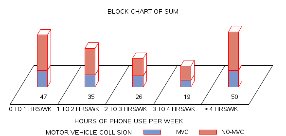
Table 17.6 Statistics for Table of Phone Use by Motor Vehicle Collision
| Statistic | DF | Value | Prob |
| Chi-Square | 4 | 0.5924 | 0.9639 |
| Likelihood Ratio Chi-Square | 4 | 0.5800 | 0.9653 |
| Mantel-Haenszel Chi-Square | 1 | 0.0327 | 0.8566 |
| Phi Coefficient | 0.0579 | ||
| Contingency Coefficient | 0.0578 | ||
| Cramer’s V | 0.0579 |
[1] From Issar, Kadakia, Tsahakis, Yoneda et al (2013): The link between texting and motor vehicle collision frequency in the orthopaedic trauma population. J Inj Violence Res. 2013 Jun; 5(2): 95-100.
