
Analysis of Non-Parametric Outcomes
22 Calculating Probabilities
Learner Outcomes
After reading this chapter you should be able to:
- apply probabilistic approaches to compute the likelihood of outcomes
- recognize and apply the binomial probability formula
1. Computing Bernoulli Trials
The rules of a Bernoulli trial are straight-forward. Given an independent process in which an outcome can be observed, the outcome can have only two possibilities and the chance or probability of the observed outcome is the same as the chance or probability of the non-observed outcome. Hence the fair toss of a fair coin is an excellent demonstration of a Bernoulli trial, because, as we observe in the tossing of a fair coin, there are only two possible outcomes: a head or a tail. Likewise, the probability of tossing a head is equal to the probability of tossing a tail, and this probability is equal to 0.5 or one-half. Further, if the coin is fair and the toss or flip is fair – without any external influence, then we can say that the process was independent.
When we are computing Bernoulli trials we often use the term event to refer to the process or test that we are conducting, and the outcome variable as the indicator variable. The outcome of an event in a Bernoulli trial is an element of the Bernoulli distribution, whereby the Bernoulli distribution is described as a discrete distribution with a possibility of one of two outcomes. The indicator variable sometimes referred to as a DUMMY variable or a BINARY variable, has two possible outcomes (success or failure). Further, when scoring the indicator variable we typically assign a value of 1 to the success and a value of 0 to the failure.
The notation used to represent the outcome of a Bernoulli trial is [latex]X_{i}[/latex], so that [latex]X_{1}[/latex] refers to a single Bernoulli trial and[latex]X_{n}[/latex] refers to n Bernoulli trials where n ranges from 1 to infinity. Further, the probability of success of an outcome in a Bernoulli trial is written as: ([latex]P(X_{i} =1)[/latex] ) = p, while the probability of failure of an outcome in a Bernoulli trial is written as ([latex]P(X_{i} =0)[/latex] ) = 1 – p.
We can also use p and q to represent the outcome of a Bernoulli trial, where p is representative of the probability of success and q is representative of the probability of failure. The probability of p is assigned in a fair and independent event as p = 0.5, and the probability of q is assigned as (1 – p) = (1 – 0.5) = 0.5.
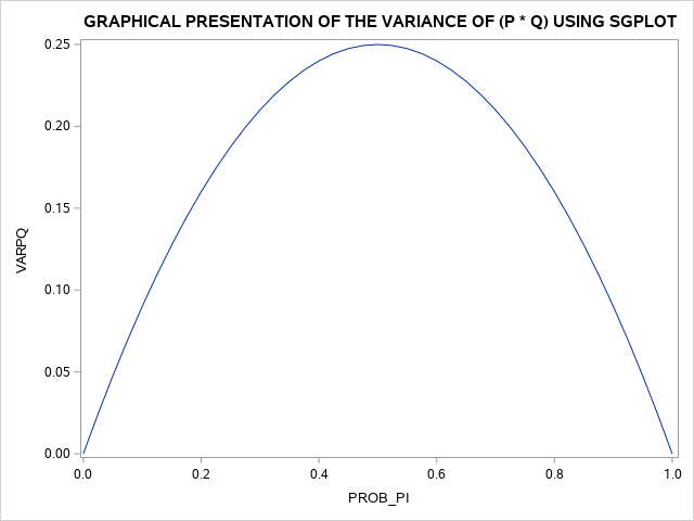
In the following example, we can use SAS and a set of probability outcomes that range from 0 to 1 and are based on an interval of 0.025 to plot the variance of a Bernoulli trial. In this example, the outcome is based on the assumption that the mean [latex]X_{i}[/latex] = p and the variance of [latex]X_{i}[/latex] = p(1-p).
The data set for this example will be based on[latex]X_{1}[/latex] = p: 0.00, 0.025, 0.05, 0.075, 0.1, 0.125, 0.15, 0.175, 0.2, 0.225, 0.25, 0.275, 0.3, 0.325, 0.35, 0.375, 0.4, 0.425, 0.45, 0.475, 0.5, 0.525, 0.55, 0.575, 0.6, 0.625, 0.65, 0.675, 0.7, 0.725, 0.75, 0.775, 0.8, 0.825, 0.85, 0.875, 0.9, 0.925, 0.95, 0.975, 1
These data are entered as follows:
1 0.00
2 0.025
3 0.05
. .
. .
. .
39 0.95
40 0.975
41 1.00
The SAS code to produce the variance [latex]\color{dbeeff}\rightarrow {varX_{1}}[/latex]= p(1-p) based on these data is shown here.
SAS Program to compute variance of a Bernoulli Trial
DATA BERNOULLI;
INPUT ID PROB_PI @@ ;
PROB_QI=(1-PROB_PI);
VARPQ=(PROB_PI * PROB_QI);
DATALINES;
1 0.00 2 0.025 3 0.05 4 0.075 5 0.1 6 0.125 7 0.15
8 0.175 9 0.2 10 0.225 11 0.25 12 0.275 13 0.3
14 0.325 15 0.35 16 0.375 17 0.4 18 0.425 19 0.45
20 0.475 21 0.5 22 0.525 23 0.55 24 0.575 25 0.6
26 0.625 27 0.65 28 0.675 29 .7 30 0.725 31 0.75
32 0.775 33 0.8 34 0.825 35 0.85 36 0.875 37 0.9
38 0.925 39 0.95 40 0.975 41 1
;
PROC SGPLOT;
SERIES X=PROB_PI Y=VARPQ;
* XAXIS TYPE = DISCRETE;
TITLE1 “GRAPHICAL PRESENTATION OF THE VARIANCE OF (P * Q) USING SGPLOT “;
RUN;
PROC PRINT;
VAR PROB_PI PROB_QI VARPQ;
TITLE1 ‘PRINT OF DATA FOR COMPLETE BERNOULLI TRIAL’;
RUN;
The SAS statements: proc SGPLOT and PLOT varpq*prob_pi produced the following graph which shows the distribution of variance across all estimates of [latex]p_{success}[/latex] and [latex]q_{failures}[/latex] from 0.00 to 1.00.
With the PROC PRINT statement, we can produce a complete listing of the data set for probabilities of success ([latex]p_{i}[/latex]) and the probability of failures ([latex]q_{i}[/latex] along with the variance of the success and failures (variance of p*q). These results are shown in the 22.1 below.
Table 22.1 Discrete Probability Distribution of the Bernouli Trial for all possible outcomes for the data set [latex]X_{i}[/latex] where i = 0 to 41.
| Obs(i) | [latex]p_{i}[/latex] | [latex]q_{i}[/latex] | variance of p*q |
| 1 | 0.000 | 1.000 | 0.00000 |
| 2 | 0.025 | 0.975 | 0.02438 |
| 3 | 0.050 | 0.950 | 0.04750 |
| 4 | 0.075 | 0.925 | 0.06938 |
| 5 | 0.100 | 0.900 | 0.09000 |
| 6 | 0.125 | 0.875 | 0.10938 |
| 7 | 0.150 | 0.850 | 0.12750 |
| 8 | 0.175 | 0.825 | 0.14438 |
| 9 | 0.200 | 0.800 | 0.16000 |
| 10 | 0.225 | 0.775 | 0.17438 |
| 11 | 0.250 | 0.750 | 0.18750 |
| 12 | 0.275 | 0.725 | 0.19938 |
| 13 | 0.300 | 0.700 | 0.21000 |
| 14 | 0.325 | 0.675 | 0.21938 |
| 15 | 0.350 | 0.650 | 0.22750 |
| 16 | 0.375 | 0.625 | 0.23438 |
| 17 | 0.400 | 0.600 | 0.24000 |
| 18 | 0.425 | 0.575 | 0.24438 |
| 19 | 0.450 | 0.550 | 0.24750 |
| 20 | 0.475 | 0.525 | 0.24938 |
| 21 | 0.500 | 0.500 | 0.25000 |
| 22 | 0.525 | 0.475 | 0.24938 |
| 23 | 0.550 | 0.450 | 0.24750 |
| 24 | 0.575 | 0.425 | 0.24438 |
| 25 | 0.600 | 0.400 | 0.24000 |
| 26 | 0.625 | 0.375 | 0.23438 |
| 27 | 0.650 | 0.350 | 0.22750 |
| 28 | 0.675 | 0.325 | 0.21938 |
| 29 | 0.700 | 0.300 | 0.21000 |
| 30 | 0.725 | 0.275 | 0.19938 |
| 31 | 0.750 | 0.250 | 0.18750 |
| 32 | 0.775 | 0.225 | 0.17438 |
| 33 | 0.800 | 0.200 | 0.16000 |
| 34 | 0.825 | 0.175 | 0.14438 |
| 35 | 0.850 | 0.150 | 0.12750 |
| 36 | 0.875 | 0.125 | 0.10938 |
| 37 | 0.900 | 0.100 | 0.09000 |
| 38 | 0.925 | 0.075 | 0.06937 |
| 39 | 0.950 | 0.050 | 0.04750 |
| 40 | 0.975 | 0.025 | 0.02438 |
| 41 | 1.000 | 0.000 | 0.00000 |
The proc freq procedure produced a complete frequency distribution independently for each of the variables: prob_pi , prob_qi , and varpq.
The output shown below is identical for the frequency distributions of the variables prob_pi and prob_qi. Therefore, only the data for prob_pi is shown here.
| prob_pi | Freq | PCT | Cumulative Frequency |
Cumulative Percent |
| 0 | 1 | 2.44 | 1 | 2.44 |
| 0.025 | 1 | 2.44 | 2 | 4.88 |
| 0.05 | 1 | 2.44 | 3 | 7.32 |
| 0.075 | 1 | 2.44 | 4 | 9.76 |
| 0.1 | 1 | 2.44 | 5 | 12.20 |
| 0.125 | 1 | 2.44 | 6 | 14.63 |
| 0.15 | 1 | 2.44 | 7 | 17.07 |
| 0.175 | 1 | 2.44 | 8 | 19.51 |
| 0.2 | 1 | 2.44 | 9 | 21.95 |
| 0.225 | 1 | 2.44 | 10 | 24.39 |
| 0.25 | 1 | 2.44 | 11 | 26.83 |
| 0.275 | 1 | 2.44 | 12 | 29.27 |
| 0.3 | 1 | 2.44 | 13 | 31.71 |
| 0.325 | 1 | 2.44 | 14 | 34.15 |
| 0.35 | 1 | 2.44 | 15 | 36.59 |
| 0.375 | 1 | 2.44 | 16 | 39.02 |
| 0.4 | 1 | 2.44 | 17 | 41.46 |
| 0.425 | 1 | 2.44 | 18 | 43.90 |
| 0.45 | 1 | 2.44 | 19 | 46.34 |
| 0.475 | 1 | 2.44 | 20 | 48.78 |
| 0.5 | 1 | 2.44 | 21 | 51.22 |
| 0.525 | 1 | 2.44 | 22 | 53.66 |
| 0.55 | 1 | 2.44 | 23 | 56.10 |
| 0.575 | 1 | 2.44 | 24 | 58.54 |
| 0.6 | 1 | 2.44 | 25 | 60.98 |
| 0.625 | 1 | 2.44 | 26 | 63.41 |
| 0.65 | 1 | 2.44 | 27 | 65.85 |
| 0.675 | 1 | 2.44 | 28 | 68.29 |
| 0.7 | 1 | 2.44 | 29 | 70.73 |
| 0.725 | 1 | 2.44 | 30 | 73.17 |
| 0.75 | 1 | 2.44 | 31 | 75.61 |
| 0.775 | 1 | 2.44 | 32 | 78.05 |
| 0.8 | 1 | 2.44 | 33 | 80.49 |
| 0.825 | 1 | 2.44 | 34 | 82.93 |
| 0.85 | 1 | 2.44 | 35 | 85.37 |
| 0.875 | 1 | 2.44 | 36 | 87.80 |
| 0.9 | 1 | 2.44 | 37 | 90.24 |
| 0.925 | 1 | 2.44 | 38 | 92.68 |
| 0.95 | 1 | 2.44 | 39 | 95.12 |
| 0.975 | 1 | 2.44 | 40 | 97.56 |
| 1 | 1 | 2.44 | 41 | 100.00 |
However, the frequency distribution for var(PQ) is unique and is shown here.
| Var(p*q) | Frequency | PCT | Cumulative Frequency |
Cumulative Percent |
| 0 | 2 | 4.88 | 2 | 4.88 |
| 0.024 | 2 | 4.88 | 4 | 9.76 |
| 0.048 | 2 | 4.88 | 6 | 14.63 |
| 0.069 | 2 | 4.88 | 8 | 19.51 |
| 0.09 | 2 | 4.88 | 10 | 24.39 |
| 0.109 | 2 | 4.88 | 12 | 29.27 |
| 0.128 | 2 | 4.88 | 14 | 34.15 |
| 0.144 | 2 | 4.88 | 16 | 39.02 |
| 0.16 | 2 | 4.88 | 18 | 43.90 |
| 0.174 | 2 | 4.88 | 20 | 48.78 |
| 0.188 | 2 | 4.88 | 22 | 53.66 |
| 0.199 | 2 | 4.88 | 24 | 58.54 |
| 0.21 | 2 | 4.88 | 26 | 63.41 |
| 0.219 | 2 | 4.88 | 28 | 68.29 |
| 0.228 | 2 | 4.88 | 30 | 73.17 |
| 0.375 | 2 | 4.88 | 32 | 78.05 |
| 0.24 | 2 | 4.88 | 34 | 82.93 |
| 0.244 | 2 | 4.88 | 36 | 87.80 |
| 0.248 | 2 | 4.88 | 38 | 92.68 |
| 0.249 | 2 | 4.88 | 40 | 97.56 |
| 0.25 | 1 | 2.44 | 41 | 100.00 |
2. The Coin Toss That Might Mean Something
The American Football league’s national championship: the Super Bowl begins with a coin toss. At the start of the game, the captain’s of each team meet in the centre of the field to toss a coin to determine which one of the teams will start the game as the kicking team and which team will start the game as the receiving team. Since the outcome of either kicking the ball to the opposing team to start the game or receiving the ball from the opposing team to start the game may have consequences on the final score, there is an attempt to make this decision an unbiased and fair process. The National Football League has chosen to render this decision to a Bernoulli trial.
Considering that a fair toss of a fair coin has a 50% chance of turning up heads and a 50% chance of turning up tails then the use of a coin toss to determine outcomes is a good approach.
The Binomial Formula establishes the probability using the following formula:
[latex]P_{x} = \frac{n!}{x!(n-x)!} \times p^{x} q^{n-x}[/latex]
The elements of this probability prediction formula are explained as follows:
[latex]P_{x} =[/latex] the probability of exactly x events of a given outcome appearing in n trials.
p = the probability of an event on any given trial (if we are flipping a coin then this value is ½ with a fair coin).
q = the probability of an event on any given trial q = 1- p (usually this value is ½ if we were flipping a coin).
n = the number of events.
x = the number of a given outcome (e.g. heads) being evaluated.
Consider an example for the Probabilities associated with tossing a fair coin
The coin tossing exercise is a useful way of demonstrating the probability of an outcome within a given set of trials when the expected chance of an outcome is fixed (known) or expected. For example, if we have a “fair” coin then the expected probability or chance of tossing a given outcome (i.e. heads) is 0.5 or ½. Therefore, given ten tosses of the fair coin we could predict the number of times we should expect to see the outcome as heads or tails.
In other words, to compute the proportion of outcomes observed we can predict the chance that an outcome or event will occur.
In the following example, we can determine the probability associated with flipping a “head” four times in ten tosses of a fair coin. That is, if we flip a fair coin ten times then we could predict the number of times we should expect to see “heads” appear in four of the ten flips.
The formula used to resolve this question is the binomial and is worked through as follows. Let x=4 (the number of heads), n=10 (the number of throws), and P=probability of 4 heads in 10 throws, where p is the starting probability and q is 1 – p. We begin with the binomial formula:
[latex]P_{x} = \frac{n!}{x!(n-x)!} \times p^{x} q^{n-x}[/latex]
Step 1: [latex]P_{4} = \frac{10!}{4!(10-4)!} \times (0.5)^{4} (0.5)^{10-4}[/latex]
Step 2: [latex]P_{4} =[/latex][latex]({10*9*8*7*6*5*4*3*2*1})\over({4*3*2*1}) \times ({6*5*4*3*2*1})[/latex][latex]\times (\frac{1}{2})^{4+6}[/latex]
Step 3: [latex]P_{4} =[/latex][latex]({10*9*8*7} \times{\enclose{horizontalstrike}{6*5*4*3*2*1}}) \over({4*3*2*1}) \times {\enclose{horizontalstrike}{6*5*4*3*2*1}})[/latex][latex]\times (\frac{1}{2})^{10}[/latex]
Step 4: [latex]P_{4} ={5040 \over{24} } \times {(1)^{10} \over (2)^{10} }[/latex]
Step 5: [latex]P_{4} ={210\times{1\over{1024} }}[/latex]
Step 6: [latex]P_{4} ={210\over{1024} }[/latex] = 0.206
The calculation table above shows us that in ten tosses of a fair coin there is roughly a 20 percent chance of tossing 4 heads. Further, we can use the binomial formula to compute all possible outcomes for a given series of events when we establish the beforehand (a priori) probability of an outcome in a defined set.
For example, let’s use the binomial to compute all possible outcomes for ten tosses of a fair coin. That is, how many times in 10 tosses would 0 heads appear? Likewise, how many times in 10 tosses would 1 through to 10 heads appear?
After working through each application of the binomial equation we could create a table of all possible events in the outcome space. This table is referred to as the Probability Density Chart, and is shown below.
The Probability Density Chart for the outcome space when determining the likelihood of tossing a head in 10 tosses of a fair coin
(x = number of a given outcome; p = ½ and q = 1 – p= ½)
| SUM | 1024:1024 | 1.00 |
| x | The probability expressed as a ratio | The probability expressed as a decimal |
| 0 | 1:1024 | 0.0009765 |
| 1 | 10:1024 | 0.0097656 |
| 2 | 45:1024 | 0.0439453 |
| 3 | 120:1024 | 0.1171875 |
| 4 | 210:1024 | 0.2050781 |
| 5 | 252:1024 | 0.2460937 |
| 6 | 210:1024 | 0.2050781 |
| 7 | 120:1024 | 0.1171875 |
| 8 | 45:1024 | 0.0439453 |
| 9 | 10:1024 | 0.0097656 |
| 10 | 1:1024 | 0.0009765 |
3. Patients as Coins – An Application of the Coin Toss
We can use the example of tossing a fair coin as a proxy for estimating the likelihood of identifying individuals to develop health conditions.
For example, consider the hypothetical situation where it is suspected that families within certain rural environments may be exposed to carcinogenic compounds in their drinking water as a result of run-off from farm fields into their wells. Let’s start with the following scenario in which you are asked, “What is the likelihood of observing 15 blood screens that test positive for a given carcinogenic substance in blood samples drawn from 25 mothers attending a prenatal health program?”
To compute the likelihood of observing 15 positive blood screens for the 25 mothers sampled, we decide to use the binomial formula with the following elements. Since we observed 15 positive cases then the term [latex]P_{x}[/latex] refers to the probability of observing this outcome in the 25 mothers, where x=15 and n=25.
[latex]P_{x} = \frac{n!}{x!(n-x)!} \times p^{x} q^{n-x}[/latex]
Step 1: [latex]P_{15} = \frac{25!}{15!(25-15)!} \times {\left({1\over{2} }\right)^{15}}{\left({1\over{2} }\right)^{25-15}}[/latex]
Step 2: [latex]P_{15} = \frac{25!}{15!\times(10!)} \times {\left({1\over{2} }\right)^{15+10}}[/latex]
While this formula looks neat in the arrangement of terms it can become quite unwieldy quickly because we are multiplying and dividing such large numbers. Note the term (n!) is 25! which indicates that we use a series of multiplication steps that are (n * (n-1)) repeatedly until we converge to (2 * (2-1)). Given that we include factorials in the numerator and the denominator our challenge is to organize all of the operations while respecting the BEDMAS principle and arriving at the appropriate solution to the formula. While we can do this with a handheld calculator it is so much easier to simply write a program to analyze this scenario using the following SAS code:
Use SAS to do the work in our computations of probability to identify individuals to develop health conditions.
DATA BERN2;
/* create the variable to represent the numerator (n!) */
NUM1 = FACT(25);/* create the variable to represent the denominator (x!(n-x)!) */
DEN1= (FACT(15)*FACT(10));/* notice in the statements above, the function to produce a factorial of a number is FACT(#), as in FACT(25) will produce the factorial of the number 25. *//* create the variable to represent the first fraction */
FRACTION1= NUM1 / DEN1;/* create variable to represent the combined probability estimates, then include PUT statement to use the outcome in the subsequent calculations */
PQ1= (0.5)**25; PUT PQ1;/* variable to represent the expected outcome */
ANSWER1 = (FRACTION1 * PQ1);
RUN;/* print the important variables */
PROC PRINT; VAR NUM1 DEN1 FRACTION1 PQ1 ANSWER1;
RUN;
The SAS code above produced the following table of results.
| 1 | 1.5511_E25 | 4.7453_E18 | 3268760 | 2.9802_E-8 | 0.097417 |
|---|
Let’s walk through this SAS Output to explain each of the parts of the exercise in calculating the probability of identifying 15 Cases from a sample of 25 women visiting the health clinic. The following elements of the Bernoulli equation (binomial equation) were computed with the SAS program above.
(i) The Numerator term is:[latex]\color{#330099}(n!)[/latex]
| 1.5511(E25) [latex]\rightarrow[/latex] reminds us to add 21 trailing zeros and move the decimal place to the right by 25 spaces, since E25 refers to 1.5511 times ten to the twenty-fifth power |
(ii) The Denominator term is:[latex]\color{#330099}(x!)\times(n-x)![/latex]
| 4.7453(E18) [latex]\rightarrow[/latex]add 13 leading zeros since E18 refers to 4.7453 times ten to the eighteenth power |
(iii) The fraction of [latex]\color{#330099}\frac{(n!)}{(x!)\times(n-x)! }[/latex] is:
| [latex]{\textit{1.5511(E25)}\over{\textit{4.7453(E18)}}} = 3,268,760[/latex] |
(iv) The unbiased expected probability terms [latex]p^x q^{n-x}[/latex] are:
| [latex]{\left({1\over{2} }\right)^{15+10}}[/latex] |
| 2.98 E-8 which represents 0.0000000298 because E with a – sign indicates the number by which we move the decimal to the left of the whole number and add leading zeros (0) |
(v) The resulting probability expressed in terms of a percentage:
| [latex]P_{15}\rvert (N=25)[/latex] |
| 0.097 can be expressed as 10% |
In example 1, we found that there was a 10% chance of observing 15 positive screens for the suspected carcinogen in the sample of 25 women attending the prenatal class.
What is the likelihood of identifying 5 positive cases for the suspected carcinogen in a sample of 50 women selected at random from the corresponding urban environment?
The SAS code to resolve this question is:
DATA BERN3;
EX2A= FACT(50); EX2B= ((FACT(5)*FACT(45)));
EX2C= EX2A/EX2B; EX2D = (0.5)**50; EX2E = EX2C * EX2D;
RUN;
PROC PRINT; VAR EX2A EX2B EX2C EX2D EX2E ;
RUN;
The SAS code produced the following output:
| Numerator [latex](50!)= 50 \times 49 \times 48 \times ... \times 2 \times 1[/latex] |
Denominator [latex](5!) \times (45!)[/latex] |
[latex]{Numerator}\over{Denominator}[/latex] | [latex]{\left({1\over{2} }\right)^{5+45}}[/latex] | [latex]P_{5}\rvert (N=50)[/latex] |
| 3.0414E64 | 1.4355E58 | 2118760 | 8.8818E-16 | 1.8818E-9 |
In example 2, we suggest that the likelihood of observing 5 cases in 50 patients was extremely unlikely and is less than 1% as shown by the answer à 1.88 E-9 which translates to a probability of 0.00000000188 given a sample size of 50 women, and can be written as: [latex]P_{5}\rvert (N=50) = 0.00000000188[/latex]
Computing the probabilities of tossing a single die
Considering a single die — what is the probability (or chance) of rolling a given number? For example, for a single die, estimate the probability of rolling a number less than “5”.
Step 1: determine the set of all possible outcomes.
1 roll of a single die = {1, 2, 3, 4, 5, 6} = 6
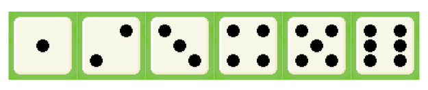
Figure 22.2 Image of all possible outcomes for a single die
On the roll of the dice . . . A single die has six sides, each side with a different number from 1 to 6.
Therefore, the set of all possible outcomes is:
– 1 die = {1, 2, 3, 4, 5, 6}
– the probability of rolling any “given number” is 1/6 or p(roll) = 0.17.
Therefore, with a single die, estimate the probability of rolling a number less than “5”.
Step 1: determine the set of all possible outcomes.
1 roll of a single die = {1, 2, 3, 4, 5, 6} = 6
Step 2: determine the set of favourable outcomes.
Numbers less than 5 = {1, 2, 3, 4} = 4
Step 3: divide the number of favourable or anticipated outcomes by the number of possible outcomes to estimate the probability. Therefore, there is a 67% chance of rolling a number less than 5 as shown here:
Probability = 4/6 = 2/3 = 0.6666 = 67%
HOWEVER, what if we were asked to consider rolling a number less than 5, in four of ten tosses of a single die? To answer this question we would apply the binomial formula, using the following apriori estimates: n=10, x=4, p=0.67, q=0.33.
[latex]P_{x} = \frac{n!}{x!(n-x)!} \times p^{x} q^{n-x}[/latex]
[latex]P_{4} = \frac{10!}{4!(10-4)!} \times {\left({0.67}\right)^{4}}{\left({0.33}\right)^{10-4}}[/latex]
[latex]P_{4} = {210} \times {0.000259}[/latex]
[latex]P_{4} = {0.05465}[/latex] = roughly 5%
4. Computing Probabilities Associated With Lottery Number Selection
So what is the probability of winning from the purchase of a single lottery ticket?
The chance of any single combination of six numbers from 1 to 49 is extremely low [latex]{1 \over {49 \choose{6}}}[/latex] which is read as 1 ticket divided by the binomial coefficient of (n choose k) or (49 choose 6) and our likelihood of winning the lottery is 1 chance in 13,983,816 combinations.
Let’s say you wanted to buy a lottery ticket on the lotto 649. You pay one dollar and pick 6 numbers from 49 on a specific computer scan sheet. Your first expectation after (or maybe prior to) purchasing the lottery ticket is that every number on the lottery card between 1 and 49 has an equally likely chance of being selected. Therefore, if every number on the card has an equally likely chance of being selected, then every combination of 6 numbers that can be made from the 49 numbers on the lottery card, has an equally likely chance of being selected. This is an expectation that the selection of the numbers from the lottery card is truly random.
How many combinations of six numbers are we really talking about?
To compute the number of possible combinations of 6 numbers from the 49 numbers, we need to use the following combinatorial (or factorial) formula. We have 49 numbers choose 6. The number 49 represents the population from which the sample “6” was chosen. We write the formula for determining the combinations using the following combinatorial equation or the binomial coefficient:
[latex]{N \choose{n}} = {49 \choose{6}}[/latex]
or we may wish to write the formula using a factorial format as:
[latex]{N! \over {n!{(N - n)}!}}[/latex] = [latex]{49! \over {6!{(49 - 6)}!}}[/latex]
Therefore the number of all possible combinations of 6 numbers from a set of 49 consecutive numbers is:
[latex]{(49 \times 48 \times ... 2 \times 1) \over{(6 \times 5 \times ... 1) \times (49 \times 48 \times ... 2 \times 1) }}[/latex][latex]= {(10,068,347,520) \over{720 }} = 13,983,816[/latex]
Yet you won’t be happy unless all of your numbers were chosen, but REALLY what is the chance that all six of your numbers will be selected by the lottery machine. Well since you only bought one ticket, then your chance of winning the lottery is 1 in 13,983,816 chances, or [latex]1 \over{49 \choose{6}}[/latex] [latex]\rightarrow { 1 \over{13,983,816} }[/latex] where the value 0.000000071 represents the probability associated with your set of scores.
Given this large set of possible outcomes, how might we evaluate the data that are generated from one year of twice-weekly draws for any patterns that seem to be emerging?
One of the simplest ways to present these data is to combine all of the numbers and present the outcome data in a chart of the frequency of outcomes. This organizational strategy would show that 6 unique numbers are drawn from the set of possible numbers ranging from 1 to 49, each week for 104 picks (52 weeks with draws held twice weekly). This approach considers that we are using sampling without replacement, which means that once a number has been selected from the set of 49 possible outcomes each week, that number cannot be selected again in that week. As shown below, the set of outcomes can be organized by the order of choices per week. That is, for any given lottery we can chart the first number drawn, the second number drawn, the third number drawn, the fourth number drawn, the fifth number drawn, or the sixth number drawn, each week.
| draw # | 1st pick | 2nd pick | 3rd pick | 4th pick | 5th pick | 6th pick |
| 1 | 13 | 21 | 7 | 32 | 47 | 11 |
| 2 | 5 | 34 | 28 | 2 | 14 | 44 |
| . | . | . | . | . | . | . |
| . | . | . | . | . | . | . |
| . | . | . | . | . | . | . |
| 103 | 33 | 16 | 21 | 48 | 15 | 1 |
| 104 | 18 | 49 | 28 | 3 | 26 | 37 |
The set of outcomes will then generate a table with 104 rows representing the six numbers drawn each week. However, this table is far too cumbersome and will not help us to make sense of the choices. Using SAS and the PROC FREQ command we can generate a set of six unique outcomes for 104 draws to replicate the twice-weekly draws of the lottery in a given year (52 weeks x 2 draws per week).
Copy the following program to your SAS space and run the program to see which lucky lottery numbers you can produce from [latex]{49 \choose{6}}[/latex]. Using if-then logic statements will enable you to group the data for each ball drawn each week and thereby provide simple categories to graph the outcomes.
SAS PROGRAM TO GENERATE 104 LOTTERY PICKS from 49 choose 6 combinations
options pagesize=60 linesize=80 center date;
PROC FORMAT;
VALUE GRPFMT 1 = ‘NUMBERS 1 TO 7’
2 = ‘NUMBERS 8 TO 14’
3 = ‘NUMBERS 15 TO 21’
4 = ‘NUMBERS 22 TO 28’
5 = ‘NUMBERS 29 TO 35’
6 = ‘NUMBERS 36 TO 42’
7 = ‘NUMBERS 43 TO 49’;
data sasrng1;
call streaminit(13);
/* this is the seed for the RNG */
array balls ball1-ball6;
do k=1 to 104;
do i=1 to 6;
balls(i) = RAND(“normal”)*1000000000000;
balls(i)=ROUND(balls(i));
balls(i)=1+(mod(balls(i),49));
balls(i) = ABS(balls(i));
if ball1 = 0 then ball1 = 1;
if ball1 >0 and ball1<8 then ball1grp=1;
if ball1 >7 and ball1<15 then ball1grp=2;
if ball1 >14 and ball1<22 then ball1grp=3;
if ball1 >21 and ball1<29 then ball1grp=4;
if ball1 >28 and ball1<36 then ball1grp=5;
if ball1 >35 and ball1<43 then ball1grp=6;
if ball1 >42 and ball1<50 then ball1grp=7;
end;
call streaminit(999);
do until (ball2 ne ball1);
ball2 = RAND(“normal”)*1000000000000;
ball2 = ROUND(ball2);
ball2 = 1+(mod(ball2,49));
ball2 = ABS(ball2);
if ball2 = 0 then ball2 = 1;
if ball2 >0 and ball2<8 then ball2grp=1;
if ball2 >7 and ball2<15 then ball2grp=2;
if ball2 >14 and ball2<22 then ball2grp=3;
if ball2 >21 and ball2<29 then ball2grp=4;
if ball2 >28 and ball2<36 then ball2grp=5;
if ball2 >35 and ball2<43 then ball2grp=6;
if ball2 >42 and ball2<50 then ball2grp=7;
end;
call streaminit(28);
do until (ball3 ne ball2 and ball3 ne ball1);
ball3 = RAND(“normal”)*1000000000000;
ball3 = ROUND(ball3);
ball3 = 1+(mod(ball3,49));
ball3 = ABS(ball3);
if ball3 = 0 then ball3 = 1;
if ball3 >0 and ball3<8 then ball3grp=1;
if ball3 >7 and ball3<15 then ball3grp=2;
if ball3 >14 and ball3<22 then ball3grp=3;
if ball3 >21 and ball3<29 then ball3grp=4;
if ball3 >28 and ball3<36 then ball3grp=5;
if ball3 >35 and ball3<43 then ball3grp=6;
if ball3 >42 and ball3<50 then ball3grp=7;
end;
call streaminit(218);
do until (ball4 ne ball3 and ball4 ne ball2 and ball4 ne ball1);
ball4 = RAND(“normal”)*1000000000000;
ball4 = ROUND(ball4);
ball4 = 1+(mod(ball4,49));
ball4 = ABS(ball4);
if ball4 = 0 then ball4 = 1;
if ball4 >0 and ball4<8 then ball4grp=1;
if ball4 >7 and ball4<15 then ball4grp=2;
if ball4 >14 and ball4<22 then ball4grp=3;
if ball4 >21 and ball4<29 then ball4grp=4;
if ball4 >28 and ball4<36 then ball4grp=5;
if ball4 >35 and ball4<43 then ball4grp=6;
if ball4 >42 and ball4<50 then ball4grp=7;
end; call streaminit(28);
do until (ball5 ne ball4 and ball5 ne ball3 and ball5 ne ball2 and ball5 ne ball1);
ball5 = RAND(“normal”)*1000000000000;
ball5 = ROUND(ball5);
ball5 = 1+(mod(ball5,49));
ball5 = ABS(ball5);
if ball5 = 0 then ball5 = 1;
if ball5 >0 and ball5<8 then ball5grp=1;
if ball5 >7 and ball5<15 then ball5grp=2;
if ball5 >14 and ball5<22 then ball5grp=3;
if ball5 >21 and ball5<29 then ball5grp=4;
if ball5 >28 and ball5<36 then ball5grp=5;
if ball5 >35 and ball5<43 then ball5grp=6;
if ball5 >42 and ball5<50 then ball5grp=7;
end; call streaminit(68);
do until (ball6 ne ball5 and ball6 ne ball4 and ball6 ne ball3 and ball6 ne ball2 and ball6 ne ball1);
ball6 = RAND(“normal”)*1000000000000;
ball6 = ROUND(ball6);
ball6 = 1+(mod(ball6,49));
ball6 = ABS(ball6);
if ball6 = 0 then ball6 = 1;
if ball6 >0 and ball6<8 then ball6grp=1;
if ball6 >7 and ball6<15 then ball6grp=2;
if ball6 >14 and ball6<22 then ball6grp=3;
if ball6 >21 and ball6<29 then ball6grp=4;
if ball6 >28 and ball6<36 then ball6grp=5;
if ball6 >35 and ball6<43 then ball6grp=6;
if ball6 >42 and ball6<50 then ball6grp=7;
end;output; end;
run;
proc freq; tables ball1grp ball2grp
ball3grp ball4grp ball5grp ball6grp;
FORMAT ball1grp — ball6grp GRPFMT. ;run;
/* CALCULATE CHI SQUARE GOODNESS OF FIT
PROC FREQ;
TABLES ball1grp/CHISQ;
FORMAT ball1grp GRPFMT. ;
TITLE ‘CALCULATING THE GOODNESS OF FIT FOR ball1grp’;
RUN; */
/* Define the axis characteristics */
axis1 offset=(0,50) minor=none;
pattern1 value=solid color=cx7c95ca;
proc sort; by ball1;
proc gchart ;
Hbar ball1grp / TYPE=PERCENT
discrete ;
FORMAT ball1grp GRPFMT. ;run;
/* Define the title */
TITLE ‘FREQUENCY DISTRIBUTION FOR OUTCOME GROUPS FOR BALL1’;
run;
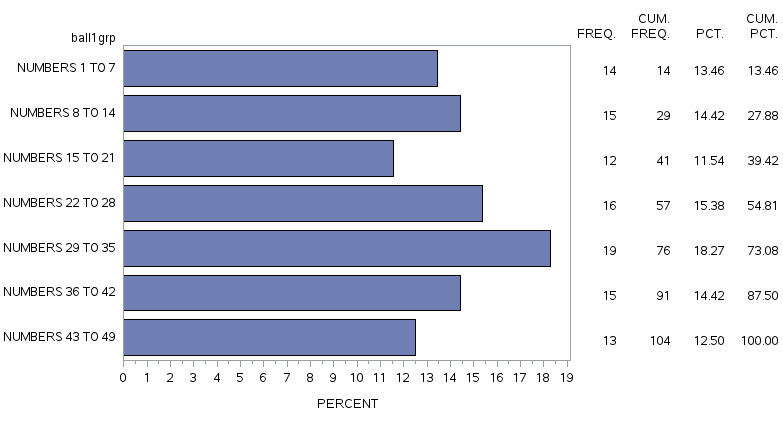
A sample of the output from this procedure is shown below:
The HORIZONTAL BARCHART WITH FREQ TABLE
