
Goodness of Fit and Related Chi-Square Tests
21 Estimating Relative Risk, the Odds Ratio, and Attributable Risk
Learner Outcomes:
After reading this chapter you should be able to:
- Assess risk for a 2 x 2 research design to test for difference in two variables measured at the nominal level
- Describe and compute the relative risk in a 2 x 2 design and specifically in a cohort study
- Describe and compute the odds ratio in a 2 x 2 design
- Describe and compute the measure of attributable risk
Assessing Risk
Computing associations with the 2 x 2 contingency table is just the beginning. In health research we are also interested in determining the extent to which an individual, having been exposed to a given circumstance or stimulus, will demonstrate an observable outcome or condition. As researchers we generate probabilistic estimates that we call risks to establish the likelihood of such stimulus-response relationships.
The term risk is classified into various estimators that help us to establish the chance of an event given a particular exposure – outcome scenario. In these next sections we will review the terms relative risk, the odds ratio, and the population attributable risk in relation to the specific webulators that assist in computing the relative estimates.
Relative Risk – Defining the term from the 2 x 2 table
A simple definition for the relative risk (RR) estimate is that it refers to the ratio of the risk of an outcome in individuals with a factor of interest to the risk of an outcome in individuals without the factor of interest. What this means is that the RR estimate is based on the relationship between two fractional estimates as shown in the following formula:
[latex]RR = {{ (a/(a+b)}\over{ (c/(c+d)}}[/latex] The relative risk formula presented here depicts the ratio of the outcomes observed among exposed individuals (a/(a+b)) to the outcomes observed among non-exposed individuals (c/(c+d)). Consider the following 2 x 2 contingency table as the starting point.
Relative risk computes the ratio of the data in cell a divided by the data in the row total of (cell a + cell b) divided by the data in cell c divided by the data in the row total of (cell c + cell d). The arrangement of the data in a, b, c, and d cells in relation to that, which is computed, is shown here.
Table 12.1 Arrangement of the data to compute Relative Risk
| Cases | Controls | ||
| Exposed | CELL “a”
+ condition + exposed |
CELL “b”
– condition + exposed |
Numerator (a/(a+b)) |
|---|---|---|---|
| Not exposed | CELL “c”
+ condition – exposed |
CELL “d”
– condition – exposed |
Denominator (c/(c+d)) |
Stated differently, the relationship between the cells in the 2 x 2 table can be explained as the ratio of the chance of an outcome among individuals who have a characteristic of interest or who have been exposed to a specific risk factor, to the chance of an outcome among individuals who lack the characteristic of interest or who have not been exposed to a specific risk factor. The relative risk estimate therefore suggests that:
The condition (or outcome) is RR times more likely to occur among those individuals that are exposed to the suspected risk factor (related to) THAN among those individuals with no exposure to the risk factor (unrelated to).
As a rule then, the larger the value of the relative risk, that is greater than 1, the stronger the association between the disease or disorder of interest and exposure to the risk factor.
Likewise, values of the relative risk estimate that are close to 1 indicate that the disease and exposure to the risk factor are unrelated (i.e., the risk of occurrence is the same for both exposed and non-exposed individuals).
Similarly values of RR less than 1 indicate a negative association between the risk factor and the disease. A relative risk estimate less than 1 is said to demonstrate a protective effect rather than a detrimental effect.
Application of The Relative Risk Estimate
In cohort studies the estimate of relative risk is used to show the ratio of the probability of those exposed versus the probability of those not exposed.
The formula for relative risk (RR) is given as the ratio of – the proportion of individuals within an exposed group showing a condition:
(cell a / (cell a + cell b))
versus the proportion of individuals within a non-exposed group showing a condition
(cell c / (cell c + cell d))
Consider The Following Example.
Researchers suggested that dental disease may be a risk factor for coronary heart disease. The suggestion in the.literature was that researchers observed the presence of a specific type of protein associated with dental disease (C-reactive protein), which may be a “cause” of myocardial infarction (i.e. heart attacks). You intend to test the relative risk of the presence of C-reactive protein on myocardial infarction by proposing the following case-control study.
Table for Relative Risk in a 2 x 2 case-control design
| Row totals | a + c = 207 | b + d = 134 | grand total= 341 |
|---|---|---|---|
| +ve condition (CASES) | -ve condition (CONTROLS) | Row Incidence | |
| Exposed | a = 186 | b = 93 | a/(a + b)
186/(186+93) =0.67 |
| Not Exposed | c = 21 | d = 41 | c/(c + d)
21/(21+41) = 0.34 |
The data in this table are used to calculate the Relative Risk as:
[latex]RR = {{ (186/(186+93)}\over{ (21/(21+41)}}[/latex]. [latex]RR = {{ (0.67)}\over{ (0.34)}}[/latex]. [latex]RR = {1.97}[/latex]
Estimating the Confidence Interval for Relative Risk in a 2 x 2 case-control design
Next we can estimate the 95% confidence estimate of this relative risk estimate (RR=1.97) using the following series of calculations.
- Convert the relative risk to natural logarithm value ln(rr) = ln(1.97) = 0.68,
- next we calculate the standard error of the ln(rr) estimate using:
[latex]{\pm z} \, {\sqrt{ { (b/a) \over (b + a)} + {(d/c) \over (d + c) } }}[/latex]
[latex]{\pm 1.96} \, {\sqrt{ { (93/186) \over (93 + 186)} + {(41/21) \over (41 + 21) } }}[/latex]
[latex]{\pm 1.96} \, {\sqrt{ { 0.002} + {0.03} }}[/latex]
Standard Error of ln(RR) = 0.35
This series of calculations produces the upper and lower limits of the 95% confidence interval for the natural logarithm of relative risk (ln(RR)).
Lower limt 95% CI ln(RR) = 0.68 – 0.35 = 0.33 and upper limt 95% CI ln(RR) = 0.68 + 0.35 = 1.03. By exponentiating the 95% confidence interval’s lower and upper limits will return the estimated values to the original scale scores, as shown here. exp(0.33) lower limt 95% CI (RR) = 1.37; and exp(1.03) upper limt 95% CI (RR) = 2.8.
Considering our decision rule whereby the larger the value of the relative risk (greater than 1) then the stronger the association between the disease or disorder of interest and exposure to the risk factor. Given a relative risk of 1.97 with upper and lover 95% confidence limits of 1.37 and 2.8, the results of your study support that the exposure C-reactive protein increases the risk of myocardial infarction. In fact, you showed that comparing the two groups, individuals suffering an MI were twice as likely to have higher levels of C-reactive protein.
Using the webulator for relative risk, we can confirm these calculations by inserting the scores into the appropriate cells of the webulator and clicking on the button labeled “Compute”.
https://health.ahs.upei.ca/webulators/rr_pb.html
We can also use the following SAS Code to evaluate the data for our C-reactive protein example.
TITLE ‘SAS CALCULATION FOR RELATIVE RISK’;
INPUT ROW COL OUTCOME @@;
DATALINES;
1 1 186 1 2 93 2 1 21 2 2 41
;
PROC SORT DATA=RROR; BY ROW COL;
PROC FREQ DATA=RROR ORDER=DATA;
TABLES ROW*COL/CHISQ RELRISK;
WEIGHT OUTCOME;
EXACT PCHI OR;
RUN;
The output generated by the SAS code is shown, below:
| Table of ROW by COL | |||
|---|---|---|---|
| ROW | COL | ||
| 1 | 2 | Total | |
| 1 |
186
54.55
66.67
89.86
|
93
27.27
33.33
69.40
|
279
81.82
|
| 2 |
21
6.16
33.87
10.14
|
41
12.02
66.13
30.60
|
62
18.18
|
| Total |
207
60.70
|
134
39.30
|
341
100.00
|
Notable output from SAS:
| Statistic | DF | Value | Prob |
| Chi-Square | 1 | 22.8723 | <.0001 |
| Phi Coefficient | 0.2590 |
| Relative Risk Estimates | |||
| Statistic | Value | 95% Confidence Limits | |
| Relative Risk | 1.9683 | 1.3766 to 2.8143 | |
Notice that the relative risk estimate and the upper and lower limits for the SAS program estimate of the 95% confidence interval of relative risk are similar to that which we calculated by hand and with the Webulator. Moreover, given that the estimate does not include a value of 1 then we can say that in comparisons between the two groups, individuals suffering an MI were nearly twice as likely to have higher levels of C-reactive protein.
Estimating the Odds Ratio
The odds ratio is another computation arising from the 2 x 2 table. Although earlier we described the odds ratio as part of the calculation for interpreting the case-control study, the odds ratio can also be used in cohort studies as well as in cross-sectional research designs, and as Bland and Altman (2002) describe are used in logistic regression analysis to evaluate the influence of measurable variables on binary relationships between variables.
Given a 2 x 2 design, as shown here, the data in Cell a refer to cases that demonstrate the condition of interest and were exposed to a suspected causal stimulus, while the data in Cell d refer to the cases that do not demonstrate the condition of interest and were likely not-exposed to the suspected causal stimulus.
Arrangement of the data to compute the Odds Ratio
| The outcome of interest Present (Cases) | The outcome of interest Absent (Controls) | ||
| Suspected causal mechanism present (Exposed) |
Cell “a”
+ case + exposed |
Cell “b”
– case + exposed |
Numerator
= (a * d) |
|---|---|---|---|
| Suspected causal mechanism absent (Not Exposed) |
Cell “c”
+ case – exposed |
Cell “d”
– case – exposed |
Denominator
= (b * c) |
The formula for the Odds Ratio is: OR = (a * d) ÷ (b * c).
As stated previously, the odds ratio is computed here to compare the ratio of cases that were exposed versus not exposed (a/c) to the ratio of non-cases among exposed versus not exposed (the control group (b/d)). The odds ratio is then the ratio of the two ratios: [(a/c) ÷ (b/d)] and can be computed by simple dividing the product of the main diagonal elements: (Cell a x Cell d) by the product of the off-diagonal elements (Cell b x Cell c).
[latex]{OR =} \, { (a \times d) \over (b \times c)} ={\textit{main diagonal elements}\over\textit{off diagonal elements} }={\textit{(+ cases, + exposed)} \times {(- cases, - exposed)}\over\textit{(- cases, + exposed)} \times {(+ cases, - exposed)}}[/latex]
So why do we call this an odds ratio?
To answer this question, let’s begin by stating what the odds ratio is not. The odds ratio is not telling us about the relative risk. To compute relative risk we looked at the proportion of cases among exposed and compared that proportion (ratio) against the proportion of cases that were not exposed. The result of the relative risk gave us the fractional comparison of cases with exposure to cases without exposure. In this way, we can say that an individual exposed to a given stimulus is RR times more likely to be a case because of the exposure.
In the odds ratio we are able to describe the likelihood associated with the outcome. Let’s put this conversation in the context of racing. To compute the odds of winning a race we need to compare the number of wins to the number of losses. If we ran five races and won three times then the odds would be calculated as: total race – number of wins = number of losses which in our example is: 5 -3 = 2. The odds are 3:2 or stated as 3 to 2.
| Computing odds | The odds of winning to losing is 3:2 |
| Number of races won | 3 |
| Number of races lost | 2 |
| Total number of races | 5 |
Now let’s return to our 2 x 2 table. The number in cell a (+cases, +exposed) are compared to the number in cell c (+cases, -exposed). The value of the (a/c) fraction can be expressed as an odds in the form a:c. Likewise, number in cell b (-cases, +exposed) are compared to the number in cell d (-cases, -exposed). The value of the (b/d) fraction can be expressed as an odds in the form b:d. Therefore, because we are computing the ratio of two odds estimates, notably, (a:c ÷ b:d) we call the estimate the ratio of the odds, or simply the odds ratio.
Estimating the Odds Ratio for a 2 x 2 table
Consider the following 2 x 2 table of the relationship between smoking status and lung cancer.
Arrangement of smoking status and lung cancer to compute the Odds Ratio
| Smoking Status | +ve condition (CASES) lung cancer present |
– ve condition (CONTROLS) no lung cancer present |
| Exposed (smoker) | cell “a” = 23
+ case, + exposed |
cell “b” = 8
– case, + exposed |
| Not Exposed (smoker) | cell “c” = 11
+ case, – exposed |
cell “d” = 25
– case, – exposed |
In this example, an individual is a member of cell “a” if they are both a smoker and were observed to be positive for lung cancer. Similarly, an individual is a member of cell “d” if they are both a non-smoker and do not show any characteristics of lung cancer. Membership in each of these cells is intuitively expected given what we know from studies of smokers and the suspected cause of lung cancer. That is if you smoke you will develop lung cancer, if you don’t smoke you won’t develop lung cancer. Seems simple enough!
However, often when describing the relationship between smoking and lung cancer, someone will undoubtedly recall a story about their grandfather that smoked his entire life but never developed lung cancer. Grandpa would, therefore, be a member of cell “b” — classified as a smoker but did not develop lung cancer. Likewise, the grandfather’s story is often countered by the story of a friend who never smoked a day in her life but died of lung cancer. This person would become a member of cell “c” – classified as a non-smoker but was observed to have developed lung cancer.
The odds ratio is computed with the following formula: OR = (cell “a” × cell “d”) ÷ (cell “c” × cell “b”). Let’s compute the ODDS RATIO by hand and then verify our computations with our webulator and with SAS.
OR = (cell A × cell D) ÷ (cell C × cell B)
OR = (23 × 25) ÷ (11 × 8)
OR = 575 ÷ 88 = 6.5
An odds ratio estimate of 6.5 suggests that individuals are 6.5 times more likely to develop lung cancer if they are classified as smokers.
Decision-making with OR and 95% confidence intervals
The odds ratio enables the researcher to test the relationship between a suspected cause and a suspected outcome by considering whether to accept or reject the null hypothesis. In its simplest form, the evaluation of an odds ratio is that there is no relationship between the suspected risk factor and the outcome, and is given by an estimate of the odds ratio to equal 1 (H0: OR=1). Some basic rules regarding the decisions about the magnitude of the odds ratio are given as follows:
- The computed odds ratio indicates to the researcher the magnitude of the suspected risk factor on the outcome condition. So that in our example we can say that a smoker is 6.5 times more likely to develop cancer if they smoke than they would by chance.
- If the computed odds ratio is close to 1 then the researcher concedes that there is no relationship between the suspected cause and the outcome.
- If the computed odds ratio is less than 1 then the researcher may suspect that the stimulus of interest is in fact demonstrating a protective effect on the sample observed.
In point 2 above, we suggested that if the odds ratio is close to 1 then the researcher concedes that there is no relationship, but how close is close to 1?
By computing confidence intervals for the odds ratio, we can determine the upper and lower bounds of the odds ratio estimate that we computed for our sample. If the 95% confidence interval includes 1 then we would say that there is no relationship between the suspected risk factor and the outcome.
In order to compute the 95% confidence interval for the odds ratio we first convert the odds ratio to its equivalent as a natural logarithm [ ln(OR)]; this is considered the point estimate for the computations of the CI. Then we compute the standard error of the natural logarithm ln(OR) by computing the square root of the sum of the inverse of each cell value as shown in the following formula (3) and then compute the 95% CI for each score. The specific calculations are shown below.
Ln(OR) = ln(6.53) = 1.88;
[latex]\textit{s.e. ln(OR) = } {\pm z} \, {\sqrt { (1/a + 1/b + 1/c + 1/d)}}[/latex]
[latex]\textit{s.e. ln(OR) = } {\pm 1.96} \, {\sqrt { (1/23 + 1/8 + 1/11 + 1/25)}}[/latex]
[latex]\textit{s.e. ln(OR) = }{\pm 1.96} \, {\sqrt{ 0.043+ 0.125 + 0.09 + 0.04}}[/latex]
[latex]\textit{s.e. ln(OR) = }{\pm 1.96} \, {\sqrt{ 0.299}} = (1.96\times 0.547) = 1.07[/latex]
[latex]\therefore[/latex] s.e. of ln(1.88) = 1.07 and the 95% C.I. for ln(OR) ± 1.96* SE ln(OR) = 1.88 +/- 1.07. Thus to compute the lower limit 95% CI we use 1.88-1.07 = 0.81 and to compute the upper limit 95% CI we use 1.88+1.07 = 2.95
Next, because the natural logarithm estimates are transformed from our original estimates we exponentiate the terms of the confidence interval estimates to return to the original scale of our data. Therefore: OR = exp(lnOR) [latex]\rightarrow[/latex] exp(1.88) so that the Odds Ratio is 6.53. Next we exponentiate the lower limit estimate: exp(LL95%) [latex]\rightarrow[/latex] exp(0.81) so that the lower limit of the 95%CI is 2.24; finally we exponentiate the upper limit estimate: exp(UL95%) [latex]\rightarrow[/latex] exp(2.95) so that the upper limit of the 95%CI is 19.10.
Elements Calculated for the 95% Confidence Interval of the Odds Ratio
| Natural Log oddsRatio ln(6.53) = 1.88 |
Standard Error of lnOR = 1.07 | 95%CI lnOR lower limit = 1.88-1.07 = 0.81 | 95%CI lnOR upper limit = 1.88+1.07 = 2.95 |
| Exponentiating the 95% Confidence Interval’s Upper and Lower limits will return the estimated values to the original scale scores | exp(0.81) = 95%CI OR lower limit = 2.24 | exp(2.95) = 95%CI OR upper limit = 19.10 |
Given that the reconstituted OR = 6.53 with a 95% confidence interval range of 2.24 to 19.10. does not include 1 then we can say that there is a relationship between the suspected risk factor and the outcome. Further, because we used 95% as the measure for our confidence interval we can say that the relationship between the suspected risk factor and the outcome is significant at the p<0.05 level.
Using the webulator for the odds ratio, we can confirm these calculations by inserting the scores into the appropriate cells of the webulator and clicking on the button labeled “Compute”.
https://health.ahs.upei.ca/webulators/or_pb.html
We can also use the following SAS Code to evaluate the data for our lung cancer and smoking example.
TITLE ‘SAS CALCULATION TO ESTIMATE THE ODDS RATIO’;
INPUT ROW COL OUTCOME @@;
DATALINES;
1 1 23 1 2 8 2 1 11 2 2 25
;
PROC SORT DATA=ODDSRAT; BY ROW COL;
PROC FREQ DATA=ODDSRAT ORDER=DATA;
TABLES ROW*COL/CHISQ RELRISK ODDSRATIO;
WEIGHT OUTCOME;
EXACT PCHI OR;
RUN;
The output generated by the SAS code is shown, below:
| Table of ROW by COL | |||
|---|---|---|---|
| ROW | COL | ||
| 1 | 2 | Total | |
| 1 |
23
34.33
74.19
67.65
|
8
11.94
25.81
24.24
|
31
46.27
|
| 2 |
11
16.42
30.56
32.35
|
25
37.31
69.44
75.76
|
36
53.73
|
| Total |
34
50.75
|
33
49.25
|
67
100.00
|
| Odds Ratio for Smoking and Lung Cancer | |||
| Statistic | Value | 95% Confidence Limits | |
| Odds Ratio | 6.5341 | 2.24 [latex]\rightarrow[/latex] 19.1 | |
Estimating Attributable Risk
According to Bruzzi, Green, Byar, Brinton and Schairer (1985)[1] a widely accepted definition of attributable risk is:
“the fraction of total disease experience in the population that would not have occurred if the effect associated with the risk factor of interest were absent”.
Quite simply stated, the attributable risk is therefore the proportion of infirmity (disease, disorder, injury, outcome) within a cohort that can be attributed to exposure to a suspected causal agent.
The attributable risk is calculated as a fraction by subtracting the proportion of cases observed among the total group of non-exposed individuals from the proportion of cases observed among the group of exposed individuals.
A caveat of this estimate is that all other possible influences of cause are considered equal among the exposed and non-exposed groups so that the only difference between the two groups is the exposure.
Attributable risk can be computed from either prevalence or incidence data and is shown here using a 2 x 2 table.
Arrangement of the data to compute Attributable Risk
| +ve condition (CASES) | – ve condition (CONTROLS) | Row totals | |
| Exposed | a | b | (a+b) |
| Not Exposed | c | d | (c+d) |
| Column totals | (a+c) | (b+d) | N= (a+b+c+d) |
| Formula for Attributable Risk | [latex]AR = P_{1} - P_{2} = {a \over(a+b)} - {c\over (c+d)}[/latex] |
||
| The formula for Attributable Risk Fraction (exposed) | 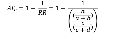 |
||
The table above illustrates the elements required to calculate the Attributable Risk Fraction (exposed)
The attributable risk fraction for exposure can be estimated from the formula shown above which includes the estimate for relative risk.
Estimating Attributable Risk for NAS Among Newborns
Consider a scenario in which 100 babies were born in the month of September, and in that cohort 11 babies were reported to show the signs Neonatal Abstinence Syndrome (NAS). As a researcher you suspect that the cause of NAS is related to the mother’s use of drugs during her pregnancy. Without sub-classifying the data according to volume or type of drug used you created the following 2 x 2 table and sorted the outcomes.
Computing Attributable Risk for NAS In Newborns
| +ve condition
(NAS CASES) |
– ve condition (CONTROLS) | Row totals | |
| Exposed – mother used a drug | 10 | 20 | 30 |
| Not Exposed – mother abstained from drug use | 2 | 68 | 70 |
| Column totals | 12 | 88 | N= 100 |
To calculate the attributable risk begin by calculating the Crude Risk Estimate for the Exposed Group: [latex]{P_{1}} = {\left(a\over{ (a+b)}\right)}= {\left(10\over{ (10+20)}\right)}= 0.33[/latex]
Next calculate the Crude Risk Estimate for the Reference Group (aka the non-exposed group): [latex]{P_{2}} = {\left(c\over{ (c+d)}\right)}= {\left(2\over{ (2+68)}\right)}= 0.029[/latex]
Attributable Risk is estimated from the proportions of outcomes based on the exposed versus non-exposed:[latex]AR = P_{1} - P_{2} = {a \over(a+b)} - {c\over (c+d)}[/latex]
[latex]AR = P_{1} - P_{2} = {10 \over(10+20)} - {2\over (2+68)} = 0.33 - 0.0285 = 0.3045[/latex]
Using the webulator shown here for attributable risk, we can confirm these calculations by inserting the scores into the appropriate cells of the webulator and clicking on the button labeled “Compute”.
https://health.ahs.upei.ca/webulators/ar_pb.html
We can also use the following SAS Code to evaluate the data for our NAS example.
The SAS code statements shown below compute the Attributable Risk as a Crude Risk in both the exposed and non-exposed – AKA reference groups. The code presented here illustrates estimates related to the attributable risk estimates, as well as estimates of the attributable risk fraction and the population attributable risk.
Title ‘Attributable Risk and Population Attibutable Risk’;
TITLE2 ‘Output includes Standardized Mortality Rate’;
input CELLA R1TOTAL CELLC R2TOTAL;
LABEL CELLA = ‘NAS POSITIVE’
R1TOTAL = ‘TOTAL EXPOSED’
CELLC = ‘NOT EXPOSED NAS POSITIVE’
R2TOTAL = ‘TOTAL NOT EXPOSED’;
DATALINES;
10 30 2 70
;
PROC STDRATE data=ARP
REFDATA =ARP
method=Indirect(AF)
STAT=RISK
Cl=normal
;
POPULATION EVENT=CELLA TOTAL = R1TOTAL;
REFERENCE EVENT = CELLC TOTAL = R2TOTAL ;
RUN ;
The SAS code above produces several measures associated with the estimates of attributable risk including the standardized mortality rate and the confidence intervals of the attributable risk.
Crude Risk Estimate from the SAS OUTPUT TABLE:
| Standardized Risk | |||
| RiskEstimate | Standard Error |
95% Normal Confidence Limits | |
| 0.3333 | 0.0861 | 0.1646 | 0.5020 |
Notice the values presented in the output table are similar to the values computed by hand and with the Attributable Risk Webulator, allowing for slight rounding differences.
SAS also reports the SMR in the table, and the calculation of the attributable risk fraction and the population attributable risk are based on the relative risk or risk ratio estimates as shown in the formula above. The method used to compute the confidence intervals for the attributable risk fraction and the population attributable risk in percentage terms are shown below.
SAS OUTPUT FOR ATTRIBUTABLE RISK
| Observed Events | Number of Obs | Crude Risk | Reference Crude Risk | Expected Events | SMR* | Standardized Risk Estimate | Standard Error | 95% Normal Confidence Limits |
|---|---|---|---|---|---|---|---|---|
| 10 | 30 | 0.33 | 0.028 | 0.857 | 11.66 | 0.33 | 0.086 | 0.164 TO 0.502 |
This table presents the output from the SAS calculations of attributable risk. The format of the table presented here differs from that which is produced by SAS but the data are the same.
The 95% confidence interval in this instance provides the range in which we are 95% confident that the true population estimate for the attributable risk is captured within the estimated interval. To calculate the confidence interval associated with the estimated attributable risk we first identify the proportions of interest from our 2 x 2 table and then compute the standard error of the difference between the two estimates. In the example used here, our proportion estimates were: [latex]P_{1} = {10 \over(30)} = 0.33[/latex] and [latex]P_{2} = {2 \over(70)} = 0.03[/latex] [latex]{\therefore} P_{1} -P_{2} = (0.33 - 0.03) = 0.30[/latex]
Next we compute: [latex]q_{1} = (1 - P_{1})[/latex] = 1-0.33 = 0.67 and [latex]q_{2} = (1 - P_{2})[/latex] = 1-0.03 = 0.97
We can now estimate the Standard Error of the Attributable Risk using:
[latex]s.e._{p_{1} - p_{2}} = {\sqrt{{{ p_{1} \times q_{1}}\over{(a+b)} } + {{ p_{2} \times q_{2}}\over{(c+d)} }}}[/latex] = [latex]{\sqrt{{{ 0.33 \times 0.67}\over{(30)} } + {{ 0.03 \times 0.97}\over{(70)} }}}[/latex]
[latex]s.e._{p_{1} - p_{2}}[/latex]= [latex]{\sqrt{0.007 + 0.0004}}[/latex] = [latex]{\sqrt{0.0074}}[/latex] = 0.086
Notice that the standard error computed by hand supports the estimate provided by SAS and the webublator.
To compute the 95% confidence interval consistent with that which our SAS code provided for the AR=0.333, we use the standard error term to estimate the range of the 95% confidence interval for the attributable risk by multiplying 1.96 x 0.086 = 0.168 so that the estimated attributable risk can range from 0.333 ± 0.168 to be [latex]\rightarrow[/latex] lower limit = 0.164 and upper limit = 0.501.
Estimating Attributable Risk Fraction and the Population Attributable Risk
In addition, as noted above, we can also compute the Attributable Risk Fraction (ARF) for the exposed individuals by using the Relative Risk (RR), where RR is the ratio of the crude risks from the exposed to unexposed, as shown here:
Relative Risk [latex]= {\left(\textit{Crude Risk for Exposed}\over{ \textit{Crude Risk for Reference Group}}\right)}= {\left(P_{1}\over{ P_{2}}\right)}=[/latex][latex]{\left(a\over{a+b}\right)} \over{ {\left(c\over{c+d}\right)}}[/latex] [latex]= {\left(0.333\over{ 0.0285}\right)}=11.67[/latex]
Next we can compute the Attributable Risk Fraction (exposed) from the data in our 2 x 2 table using ; where a=10, b=20, c=2, d=68.
So that [latex]AF_{exposed} = 1 - {1 \over{\textit(RR)}}[/latex] = [latex]1 - {1 \over{11.67}}[/latex] = 0.9143 which we can convert to a percent value using [latex]\rightarrow[/latex] 0.9143 [latex]\times[/latex] 100.
Likewise the attributable risk can also be calculated in percentage terms using:
[latex]ARF = {P_{1}-P_{2} \over{P_{1}}} \times 100 = {0.33-0.0285 \over{0.33}} \times 100= {0.30 \over{0.33}} \times 100[/latex] = 91%
The estimated Attributable Risk Fraction (exposed) is useful because it can be interpreted relative to the effect of exposure. Here we can say that the estimate for the Attributable Risk Fraction (exposed) indicates that the risk of NAS among babies is approximately 91% higher when the mother uses a drug during pregnancy.
When we compute the Attributable Risk Fraction (exposed), a typical next step is to compute the population attributable risk (PAR). The population attributable risk is an estimate that extends the attributable risk fraction from the observed sample to the larger population.
Again, using the data from our 2 x 2 table the PAR can be calculated as follows:
[latex]PAR = p {\left((RR-1)\over{RR}\right)}; \textit{Where: } p= {\left(a\over{ (a+c)}\right)}=[/latex] [latex]{10\over{12}}= 0.833[/latex] and RR = 11.67 [latex]\therefore PAR = {10\over{12}} \times{11.67 - 1 \over{11.67}} = 0.833 \times{0.9143} =0.7642[/latex]. This value can also be expressed in percentage terms as approximately 76%.
The SAS code statements used to compute the estimates for the ARF and PAR provide a summary table that includes the population estimates for each of the parameter values. It is important to notice, that although we can use simple algebra to compute the point estimates, the confidence intervals are not normally distributed and therefore require more advanced formulae that are available on the SAS Support website.
SAS Output for Attributable Fraction Estimates
| Parameter | Estimate | 95% Confidence Limits | |
|---|---|---|---|
| Attributable Risk | 0.91429 | 0.82647 | 0.94309 |
| Population Attributable Risk | 0.76190 | 0.21732 | 0.92757 |
The important information to glean from the output table above is that because neither the estimate for the Attributable Risk Fraction nor the Population Attributable Risk includes 0, we can say that consistent with the test of the null hypothesis, these observed parameter estimates are significant at the p<0.05 level; and that taking drugs while pregnant CAN increase the risk of NAS in newborns.
[1] Bruzzi, P., S. B. Green, D. P. Byar (Biometry Branch, National Cancer Institute, NIH, Bethesda, MD 20205), L A. Brinton, and C. Schairer. Estimating the population attributable risk for multiple risk factors using case-control data. Am j Epidemiol 1985; 122:904-14.
