
Parametric Statistics
30 The t-test for Independent Sample Means and Pooled Versus Unpooled Variance
Learner Outcomes
After reading this chapter you should be able to:
- Compute the significance of the difference between two sample means when the sample variances are different
- Compute the t-test for independent sample means
- Compute the t-tests for pooled versus un-pooled variance.
- Write a SAS program to compute and identify the important elements of the output for the computation
Applications of the t-test under different research scenarios
In statistics, the t-test has a simple approach despite that it uses a variety of error terms in the denominator as shown in Table 30.1, below. Depending on the research design, the error term will differ to ensure that the appropriate variance estimates within each of the samples are included in the analyses. The following equations demonstrate the different error terms related to the types of comparisons.
Table 30.1 A Summary of t-test Formulae
| t-test descriptions | Appropriate t-test formula |
| Evaluation of the single sample mean versus the mean for a population | 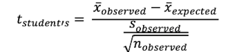 |
| The pairwise t-test uses the average difference in the measure of interest, from the pre-test score to the post-test score, and then divided by the standard error of the average difference. The standard error of the average difference is computed by dividing the standard deviation of the average difference by the square root of the number of cases in the pairwise comparison. | 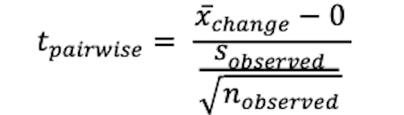 |
| To evaluate the significance of the difference between two mean scores (regardless of the size of “n” in each level of the independent variable) we might consider using a pooled t-test for independent variables. | 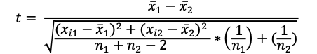 |
| To evaluate the significance of the difference between two mean scores (regardless of the sample size “n”) when we consider un-pooled or unequal variances | 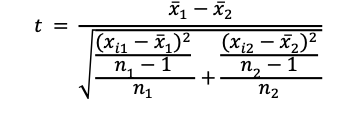 |
In Figure 30.1 below we see the two dimensions of variance that can contribute to the differences observed in a t-test calculation. As illustrated, not only does the t-test process the differences between means, but the difference is also influenced by the variability between members within each sample.
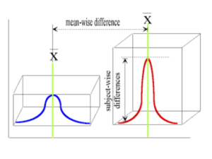
Figure 30.1 Comparison of Two Independent Means
Notice that the decision about which t-test formula to select is dependent on the research design created by the researcher. For example, as noted in table 30.1, to evaluate the significance of the difference between two mean scores (regardless of the size of “n” in each level of the independent variables) we could consider using a t-test for independent variables, as noted in Table 30.1 formula 3. However, if the number of participants in the samples being compared is equal then it is more appropriate to use Table 30.1 formula 4. In this latter case, given that the sample size between the groups was equal and it is expected that the variance within the two groups is similar. In this case, we can pool or combine the variance estimates as we assume that the two groups have homogenous variance within and between the two groups.
Scenario 30.1.1 Comparing 2 groups with unknown variance and different sample sizes
Consider the following scenario in which there are two groups with different sample sizes (number of participants in each group) and the variance is unknown within each of the groups. In this situation, the analysis of data uses the t-test for two independent groups. We can use the formula for the t-test for independent groups (with unequal sample sizes) to compute the significance of the differences in the mean scores from group1 in which the sample size is 10 participants and the mean scores from group2 where the sample size is comprised of 8 participants.
Table 30.2 Comparing Responses for two groups with unequal sample sizes and unknown variance
Data for Group 1
| Participant ID | 001 | 002 | 003 | 004 | 005 | 006 | 007 | 008 | 009 | 010 |
|---|---|---|---|---|---|---|---|---|---|---|
| Score | 234 | 254 | 260 | 268 | 253 | 270 | 281 | 287 | 265 | 255 |
Data for Group 2
| Participant ID | 001 | 002 | 003 | 004 | 005 | 006 | 007 | 008 |
|---|---|---|---|---|---|---|---|---|
| Score | 304 | 235 | 212 | 198 | 273 | 289 | 301 | 209 |
The degrees of freedom for the two-group t-test is df=n1+n2-2, and in this case df=10-8-2=16 so that the t critical value based on an alpha level of 0.05 is 2.12.
In the following SAS code, we compute the difference between the means for the data in Table 30.2. Here we include a grouping variable so that we can distinguish the data for each group before computing the t-test.
T-test for the difference between means with unequal sample size
DATA INDT_TST;
INPUT ID GROUP SCORE @@;
DATALINES;
001 1 234 002 1 254 003 1 260 004 1 268 005 1 253 006 1 270 007 1 281 008 1 287 009 1 265 010 1 255 011 2 304 012 2 235 013 2 212 014 2 198 015 2 273 016 2 289 017 2 301 018 2 209
;
PROC SORT DATA=INDT_TST; BY GROUP;
PROC TTEST; CLASS GROUP; VAR SCORE;
RUN;
The output for the PROC T-TEST procedure for this independent t-test analysis is shown below. The INDEPENDENT t-test Procedure.
| GROUP | N | MEAN | STD | STD ERR | MINIMUM | MAXIMUM |
| 1 | 10 | 262.7 | 15.17 | 4.79 | 234.0 | 287.0 |
| 2 | 8 | 252.6 | 44.02 | 15.56 | 198.0 | 304.0 |
| GROUP | MEAN | STANDARD DEVIATION |
| Diff (1-2) | 10.08 | 31.26 |
| group | Method | Mean | Std Dev |
| 1 | 262.7 | 15.17 | |
| 2 | 252.6 | 44. | |
| Diff (1-2) | Pooled | 10.0750 | 31,26 |
| Diff (1-2) | Satterthwaite | 10.0750 | 47.37 |
| Method | Variances | DF | t Value | Pr > |t| |
| Pooled | Equal | 16 | 0.68 | 0.51 |
| Satterthwaite | Unequal | 8.33 | 0.62 | 0.55 |
Equality of Variances
| Method | Num DF | Den DF | F Value | Pr > F |
| Folded F | 7 | 9 | 8.42 | 0.0049 |
To determine if the mean scores in each group were significantly different we typically compare the t-observed to the t critical values, generally available in a reference table. For example, the t critical value for α = 0.05, where df=9 is 2.262 for a two-tailed test and 1.833 for a one-tailed test. In the SAS output shown here, a t-critical is not given, however, the probability of achieving the t-value that was computed is reported and this is the indicator of significance. That is to say, when the Pr > |t| is greater than 0.05, as it is in this instance, we would accept the null hypothesis that there is no difference between the mean scores in each group.
Additionally, in the SAS output, we observe a t-value for both a pooled variance estimate and for an un-pooled variance estimate, where the Satterthwaite t Value estimates the unequal/un-pooled variance. As a general rule because the Folded F stat is a test of unequal variances, when the folded F statistic is large and the p-value is <0.05, as shown in the SAS output above, then we refer to the Satterthwaite unequal variances estimate to determine the decision rule regarding the comparison of means via the t-test.
30.2 On the importance of p-values
In the following data set there were 2 groups of 15 individuals. A test was conducted and each individual produced a score. The means were then computed for the scores in each group and a t-test was used to determine if there was a significant difference between the means for each group. The null hypothesis was given as: H0: mean for group1 = mean for group2
Data in Scenario 1:
The data for each group is shown here using the format (id, group, score):
001 01 12, 002 01 25, 003 01 26, 004 01 23, 005 01 14, 006 01 15, 007 01 17, 008 01 11, 009 01 18, 010 01 14, 021 01 25, 023 01 28, 025 01 26, 027 01 23, 029 01 24 011 02 15, 012 02 34, 013 02 39, 014 02 35, 015 02 34, 016 02 33, 017 02 15, 018 02 31, 019 02 13, 020 02 20, 022 02 16, 024 02 22, 026 02 27, 028 02 26, 030 02 25
The results of the t-test computation using SAS are shown here:
The UNIVARIATE Procedure – Data for the total group for Dependent Variable Score
| N | 30 | Sum Weights | 30 |
| Mean | 22.8666667 | Sum Observations | 686 |
| Std Deviation | 7.7135498 | Variance | 59.4988506 |
| Skewness | 0.25907362 | Kurtosis | -0.8503857 |
| Uncorrected SS | 17412 | Corrected SS | 1725.46667 |
| Coeff Variation | 33.7327251 | Std Error Mean | 1.40829508 |
The t-TEST Procedure
| group | N | Mean | Std Dev | Std Err | Minimum | Maximum |
| 1 | 15 | 20.0667 | 5.8244 | 1.5039 | 11.0000 | 28.0000 |
| 2 | 15 | 25.6667 | 8.5161 | 2.1988 | 13.0000 | 39.0000 |
| Diff (1-2) | -5.6000 | 7.2955 | 2.6639 |
| group | Method | Mean | 95% CL of the Mean | Std Dev | |
| 1 | 20.0667 | 16.8412 | 23.2921 | 5.8244 | |
| 2 | 25.6667 | 20.9506 | 30.3827 | 8.5161 | |
| Diff (1-2) | Pooled | -5.6000 | -11.0568 | -0.1432 | 7.2955 |
| Diff (1-2) | Satterthwaite | -5.6000 | -11.0893 | -0.1107 | |
| Method | Variances | DF | t Value | Pr > |t| |
| Pooled | Equal | 28 | -2.10 | 0.0447 |
| Satterthwaite | Unequal | 24.746 | -2.10 | 0.0459 |
Equality of Variances
| Method | Num DF | Den DF | F Value | Pr > F |
| Folded F | 14 | 14 | 2.14 | 0.1675 |
So for this output, we would reject the null hypothesis and suggest that the mean for Group 1 was significantly different than the mean for Group 2. However, what would happen if in one of the groups we changed one of the scores by 5 points. Notice in the following data set for Scenario 2, all of the scores are exactly the same, except that we changed the data for participant 1 from 12 to 17.
Data in Scenario 2:
The data for each group are shown here using the format (id, group, score):
001 01 17, 002 01 25, 003 01 26, 004 01 23, 005 01 14, 006 01 15, 007 01 17, 008 01 11, 009 01 18, 010 01 14, 021 01 25, 023 01 28, 025 01 26, 027 01 23, 029 01 24, 011 02 15, 012 02 34, 013 02 39, 014 02 35, 015 02 34, 016 02 33, 017 02 15, 018 02 31, 019 02 13, 020 02 20, 022 02 16, 024 02 22, 026 02 27, 028 02 26, 030 02 25
The t-test output for Scenario 2 uses the exact same data set, except that the score for participant 1 in Group 1 was changed from a score of 12 to a score of 17. Notice the highlighted t values and the highlighted confidence intervals.
| group | Method | Mean | 95% Confidence Limits for the Mean | Std Dev | |
|---|---|---|---|---|---|
| 1 | 20.4000 | 17.3755 | 23.4245 | 5.4616 | |
| 2 | 25.6667 | 20.9506 | 30.3827 | 8.5161 | |
| Diff (1-2) | Pooled | -5.2667 | -10.6175 | 0.0841 | 7.1538 |
| Diff (1-2) | Satterthwaite | -5.2667 | -10.6597 | 0.1264 | |
| Method | Variances | DF | t Value | Pr > |t| |
|---|---|---|---|---|
| Pooled | Equal | 28 | -2.02 | 0.0535 |
| Satterthwaite | Unequal | 23.85 | -2.02 | 0.0552 |
In this second example analysis, we would accept the null hypothesis indicating that there was no difference between the means. This decision is based on the comparison of the p-value to the accepted demarcation point of p<0.05.
Despite that we have a demarcation point for the probability of the observed t-test, we need to consider the range of scores that we could have seen. The confidence interval provides such information for us. In the first example, the 95% confidence interval tells us that we are 95% confident that the difference between means could be somewhere between -11.09 and -0.11. However, in the second example the 95% confidence interval tells us that we are 95% confident that the difference between means could be somewhere between -10.66 and 0.126.
Sullivan and Feinn[2] provide two quotes to support the need to look beyond the simple comparison of research findings to a p-value. The first quote is by Gene Glass who said, “Statistical significance is the least interesting thing about the results. You should describe the results in terms of measures of magnitude – not just, does a treatment affect people, but how much does it affect them.”.
The second quote is by Jacob Cohen, who said, “The primary product of a research inquiry is one or more measures of effect size, not P values.”.
Two important points of interest arise from this comparison. The first being that the intervals are not only similar in size but that they are similar in the bandwidth on the number line[latex]\;\rightarrow\;[/latex] lower limits being (-11.09 and -10.66) and upper limits being (-0.11 and 0.126). However, the second point of interest is that we only had to change one score from the entire set of 30 scores and only by 5 points in order to change from showing a significant difference to a non-significant difference.
If you consider the standard deviation for the scores in Group 1 in each trial, you will notice that a 5-point change is less than the score by which we expect any score to vary from the mean. That is, in the two examples the standard deviation is 5.82 and 5.46, respectively. Therefore, changing a score by less than the computed standard deviation was sufficient to cause a decision to change from significant to not significant.
Consider that this was a study in which you invested millions of dollars. If you only relied on the p-value then you would be happy with scenario 1 (a significant difference was found) but you would be tremendously disappointed with scenario 2, and you would unnecessarily throw away valuable information. So a guiding principle may be that despite the reported value of p for any comparison, consider also the standard deviations and the standard errors along with the computed confidence intervals before reporting the findings.
30.3 Estimating the Effect Size
We can compute the effect size – where the effect size is defined as the magnitude of the difference between the two means when the difference is adjusted by the standard deviation for the mean of interest. The formula is simply the difference between the two means in a scenario that compares two groups divided by the standard deviation of the group of interest. So how do I establish the group of interest? The confusion in using this formula is often in which standard deviation to select. One way is to simply select one group to be the standard reference group and the other group to be the group of interest.
The Effect Size formula: [latex]ES = {\left(\overline{x_{1}} - \overline{x_{2}}\right)\over{s_{1}} }[/latex]
The effect size formula is often interpreted using Cohen’s criteria where an effect size score of 0.2 is considered as a small but noticeable effect, while an effect size score of 0.5 is considered to be a medium effect size, and an effect size score of 0.8 is considered to be a large effect size.
We can also calculate the confidence interval for the difference between two means in any scenario where we compute the t-observed score. The formula to compute the confidence interval for a mean difference for two independent samples is shown here. The elements for this calculation are produced from the SAS output using PROC UNIVARIATE or PROC MEANS and substituted into the equation. The formula for confidence intervals in a t-test for independent samples is:
[latex]\left(\overline{x_{1}} - \overline{x_{2}}\right) \pm t_{0.05} \times \sqrt{\frac{s^2_{1}}{n_{1}}+ \frac{s^2_{2}}{n_{2}}}[/latex].
Where the t0.05 is the critical value for t for the degrees of freedom in the study. Considering that we have 50 cases in our sample our degrees of freedom value will be: df = (n1– 1) + (n2 – 1) and the critical value of t0.05 = 2.01
The decision rule concerning a confidence interval in a t-test for independent samples is to determine if the range of the confidence interval from the lowest value to the highest value includes 0. If 0 is included in the range then we accept the null hypothesis that the mean for group 1 = the mean for group 2.
30.4 The degrees of freedom and critical values
- The term degrees of freedom, represents the number of scores within a set of scores that are free to vary, and the number of scores that must be fixed, in order to compute a result.
For example: Consider that the average age for a group of five students is 22. Therefore, the mean of 22 is the outcome or the result. Now consider what each student’s age must be in order to calculate an average age of 22 [latex]\rightarrow\;[/latex] the outcome (aka the result).
In other words within the set of scores that we observed, what scores are required to make up the set of scores, in order to compute the outcome (result) that we observed?
Let’s work through the concept with the following example:
Identify a sample of five students and then decide to ask each student to report their age. The first student tells you that she is 28 years old, but the second student said that he is 12 years old! Student number 3 reports that he is 129 years old and the fourth student suggests that her age is a whopping -10! No doubt you are realizing that their ages are totally fictitious but they are what they are, and the outcome for the average age remains at 22. Your challenge is now to determine what the age of the fifth student is in order to ensure that the overall group age is 22. That is, the age of the student cannot be a free choice but must be a fixed age in order for you to calculate the mean age for the group equal to 22.
In this example, you have some known information. You began with the outcome as the mean age of the group equal to 22, and you also have a set of 4 age values that were reported for the group (28, 12, 129, and -10). Since you know the real average age of the five students is 22. You decide to play along with the group, and you realize that you can use simple arithmetic factoring to solve the unknown value of the age for the 5th student.
[latex]\overline{x} = {\Sigma{\left(x_{1}\; +\; x_{2}\;+\; ... \;+\; x_{n}\right)}\over{n} }[/latex] [latex]= {\Sigma{\left(28\; +\; 12\;+\; 129 \;+\; (-10)\;+\; x_{5}\right)}\over{n} }[/latex]. Work through the computation of the numerator, and then factor out the [latex]x_{5}[/latex] term by multiplying each side by the denominator value of 5, and then subtracting 159 from both sides as shown here.
| [latex]22 = {159 + x_{5}\over{5}}[/latex] | [latex]22 \times{5} = {\bcancel{5} \times \left(159 +x_{5}\right)\over{\bcancel{5}}}[/latex] | [latex]110 = \left(159 + x_{5}\right)[/latex]
[latex]110 - 159 = \left(x_{5}\right)[/latex] [latex]-49 = \left(x_{5}\right)[/latex] |
Since you know the real average age of the five students is 22. You determine that the age for Student #5 MUST BE (-49). The degrees of freedom is a term that represents the number of scores within a set of scores that are free to vary, and the number of scores that must be fixed, in order to compute a result. In your data set, 4 of the ages were free to vary, but the age for Student #5 had to be fixed at (-49) in order to compute the group’s known mean age of 22.
A simple formula for degrees of freedom is then to consider that the degrees of freedom equal the number of scores that are free to vary minus the number of scores that are fixed within a set of scores.
Why compute the DEGREES OF FREEDOM?
The degrees of freedom term is used to determine the critical value of a statistic given the research design and the sample size. In other words, the value from the probability distribution function for all possible scores of the statistic of interest under an estimate of the probability for a given research scenario. The statistic’s critical score is related to the probability that the null hypothesis is true. In the case of using the t-test, the null hypothesis is a derivative of the mean observed being equal to the mean expected. The critical value can change for every application of a statistical computation because it depends on the size of each sample and the probability level set by the researcher to establish whether or not to accept or reject the null hypothesis (i.e. the level of significance).
All degrees of freedom computations can be derived from the following formula: df = (n – 1). Below is a table of degrees of freedom formulae for different types of t-test designs. Notice that the formula differs to enable freedom of at least 1 measure within each array (set) of data.
Table 30.3 Degrees of freedom computations for different t-test designs
| TERM and Null Hypothesis | FORMULA | EXAMPLE |
| Student’s t-test
H0: sample mean = 0 |
df = (n – 1) | Given a sample size of 10, degrees of freedom is: df=(10 – 1), df = 9
|
| Pair-wise t-test
H0: preTestmean = postTestmean |
df = (npairs – 1) | Given a sample size of 10 pairs, degrees of freedom is: df=(10 – 1), df = 9
|
| t-test for two group comparisons—equal n in each group[1]
H0: grp1mean = grp2mean |
(n1 + n2) – 2 | Given that the sample sizes are n1= 10 and n2=10, degrees of freedom is:
df=(10 + 10) – 2, df = 18
|
| t-test for two group comparisons—unequal n in each group
H0: grp1mean = grp2mean |
(n1– 1) + (n2 – 1) | Given that the sample sizes are n1= 8 and n2=13, degrees of freedom is:
df=(8-1) + (13-1), df = 19
|
[1] assuming equal variances within the two sample distributions
[2] Sullivan, G , and Feinn, R., Using effect size, or why the p Value isn’t enough, Journal of Graduate Medical Education, September 2012, 279-282.
