
Advanced Concepts for Applied Statistics in Healthcare
43 Survival Analysis
Essential Background in Survival Analysis
Survival analysis can be considered in its simplest form as a method to analyze longitudinal data for a cohort, or for a comparison of cohorts with a specific interest in the proportion of individuals that reached or exceeded a definite point on a time scale.
In survival analysis, the demarcation point for the event of interest on a time scale is referred to in a variety of ways but is dependent upon the perspective of the researcher. For example, if the researcher is interested in the application of survival analysis to estimate mortality as a result of a given treatment regimen then the demarcation point may be used to count the number of individuals that died within the interval up to a specific time, versus the number of individuals that lived beyond the selected time (i.e. survived). However, given the intention of the research, the mathematics of survival analysis need not be limited to only counting deaths (or survival), rather, the approaches of survival analyses may be thought of as a set of mathematical functions that enable statistical techniques which can be applied to the evaluation of any selected event at a specific period of time. Hence, there are several methods that can be used to perform survival analysis, however, in this chapter, the focus will be on the application of SAS for survival analysis using life tables, the calculation of the log-rank test, and the application of the Cox Proportional Hazard Model.
Important Functions Used in Survival Analysis
The progression of information about functions used in the computation of survival analyses is presented in Figure 19.1. In the following section, we will review the important concepts of the probability density function for a random discrete variable and a random continuous variable, the cumulative distribution function, the survival function, and the hazard function.
The flow of function processing in survival analysis
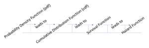
There are several ways to demonstrate survival analysis, but we will begin here by reviewing the basic terminology and the elements of the different functions used in the calculation of survival analysis so that we can measure the risk of an event happening at a specific period of time.
The probability density function represents a value that describes the probability of an outcome or a combination of outcomes occurring within a known outcome space – such as an interval.
The probability density function (pdf) can refer to either the associated probability value from a discrete random variable or from a continuous random variable. When the pdf refers to a discrete random variable then it is also referred to as the probability mass function (pmf) for a positive discrete random variable. In this case, we define a positive discrete random variable as a variable that holds numbers from the whole number line, meaning that the scores are whole numbers (ranging from 0 to + ∞) and may resemble (0,1,2,3, …, ∞) without decimal values.
Probability Density Function (pdf) Related to Tossing a Single die
| Possible outcome expressed as [latex]P(X = x)[/latex] | The probability associated with the outcome |
| [latex]P(X = 1)[/latex] | 1/6 |
| [latex]P(X = 2)[/latex] | 1/6 |
| [latex]P(X = 3)[/latex] | 1/6 |
| [latex]P(X = 4)[/latex] | 1/6 |
| [latex]P(X = 5)[/latex] | 1/6 |
| [latex]P(X = 6)[/latex] | 1/6 |
A graph of the frequency distribution for these data would produce a platykurtic (flat) distribution profile since each outcome value has a frequency of 1.
However, we could create a graph to demonstrate the cumulative outcomes for the probabilities of the random discrete variable (X) ranging from 1 to 6; which would be to consider the discrete outcome ranging as follows: Ρ(X=1) ≤ Ρ(X=6).
The Cumulative Distribution Function commonly referred to as the c.d.f. and written as F(x)=P(X≤x) represents the set of values associated with the probabilities of the random variable (X) occurring equal to or less than a given value (x) in an outcome space.
In the example of the toss of a fair six-sided die, the outcome space is based only on the discrete numbers 1 through 6, as shown in the following outcome chart.
Cumulative Distribution Function (c.d.f) Related to Tossing a Single die
| Possible outcome expressed as [latex]P(X \le x)[/latex] | Probability associated with the outcome |
| [latex]P(X \le 1)[/latex] | 1/6 = 0.17 |
| [latex]P(X \le 2)[/latex] | 2/6 = 0.33 |
| [latex]P(X \le 3)[/latex] | 3/6 = 0.50 |
| [latex]P(X \le 4)[/latex] | 4/6 = 0.67 |
| [latex]P(X \le 5)[/latex] | 5/6 = 0.83 |
| [latex]P(X \le 6)[/latex] | 6/6 = 1.00 |
While the example presented here describes the c.d.f. for discrete random variable outcomes (and their associated probabilities based on the probability mass function (pmf) or probability density function (pdf)), the c.d.f. is also relevant for continuous variable values and the pdf is based on the outcomes (X) in an interval (a, b) represented by P(a < X < b), where all numbers from the real number line are eligible within the interval of the distribution, typically ranging from 0 to 1.
If the data for the c.d.f. were attributed to a continuous random variable such as time, then the graph of the set of probabilities for all possible outcomes of the c.d.f. is presented as a positive S-shaped curve ranging from 0 to 1, as shown in the figure below.
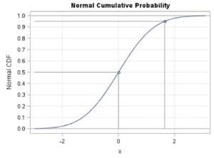
Schematic of a c.d.f. for a Continuous Random Variable
The SAS code to generate this image was written by Wicklin (2011)[1] and was processed unedited in SAS Studio shown here.
data cdf;
do x = -3 to 3 by 0.1;
y = cdf(“Normal”, x);
output; end;
x0 = 0;
cdf0 = cdf(“Normal”, x0);
output;
x0 = 1.645; cdf0 = cdf(“Normal”, x0); output;
run;
ods graphics / height=500;
proc sgplot data=cdf noautolegend;
title “Normal Cumulative Probability”;
series x=x y=y;
scatter x=x0 y=cdf0;
vector x=x0 y=cdf0 /xorigin=x0 yorigin=0 noarrowheads lineattrs=(color=gray);
vector x=x0 y=cdf0 /xorigin=-3 yorigin=cdf0 noarrowheads lineattrs=(color=gray);
xaxis grid label=”x”;
yaxis grid label=”Normal CDF” values=(0 to 1 by 0.05);
refline 0 1/ axis=y;
run;
The c.d.f. is an important step in the computation of the survival analysis because it is part of the computation of the survival function. In a time relevant model as is typical in a biostatistics application, the cumulative distribution function can be represented as [latex]F(t)=P(T \le{t}) \textit{where t}[/latex] is the value of the random variable representing a measured time and [latex]{t}[/latex] is the value of the intended time at the event.
The survival function [latex]S{(t)}[/latex] provides the estimate of the duration of time to an event, be it a failure, death, or a specified incident. The survival function begins at 1, the point where an individual enters the dataset and ends at 0 the point where data monitoring stops, usually because the event of interest has occurred.
In simple terms, the Survival Function is the complement of the c.d.f. and is computed as [latex]S{(t)}= 1- F(t)\textit{, where t >0}[/latex]. More important, the survival function is the denominator in the computation of the Hazard Function, which is a main element in one approach to the computation of the survival analysis. The survival function can show the probability of surviving up to a designated event, based on units of time.
For example, consider the following data set in which a measure of time to an event is recorded.
Table depicting number of individuals that exceeded the time to event
| Patient ID | Time to Event: The measure of the length of time to the event happening | Event Counter variable (0=event has not happened, 1=event has happened) |
| 01 | 40 | 0 |
| 02 | 38 | 0 |
| 03 | 54 | 1 |
| 04 | 56 | 1 |
| 05 | 28 | 0 |
| 06 | 36 | 0 |
| 07 | 42 | 0 |
| 08 | 51 | 1 |
| 09 | 45 | 0 |
| 10 | 49 | 1 |
The data are processed with the following SAS code[2] to produce a graph of the survival curve shown below.
title ‘program to show a survival curve’;
data survcurv;
input id t_event censor;
datalines;
01 40 0
02 38 0
03 54 1
04 56 1
05 28 0
06 36 0
07 42 0
08 51 1
09 45 0
10 49 1
;
proc lifetest data=survcurv(where=(censor=1)) method=lt
intervals=(45 to 60 by 1) plots=survival;
 time t_event*censor(0);
run;
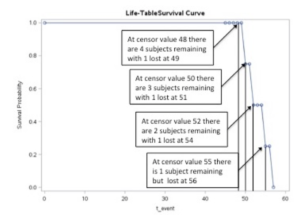
The results of this analysis include the table of the survival estimates and the survival curve below – note that the failure point was set at 48. The curve shows the probability of surviving to 48 and then beyond 48.
Notice that the entire group begins at probability = 1 and ends at probability = 0.
Figure of SAS representation of the survival function for n=10 with censoring at x=48.
The Hazard Function is determined by the ratio of the probability density function (pdf) to the survival function [latex]S{(t)}[/latex] and can be written as:[latex]\lambda = {(p.d.f.) \over{S(t)}}[/latex]
The following explanation may help to describe the elements of the hazard function in greater detail. In this annotated formula the hazard function is shown to represent the likelihood of an event such as death or survival occurring within an interval at time [latex]{(t)}[/latex].
[latex]\lambda(t) = {\lim\limits_{\Delta{t}\to {0}}} {P(t \le{T} \lt{t} + \Delta{t} \mid{T} \ge{t})\over{\Delta(t)}}[/latex]
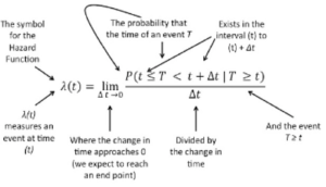
Annotated image of the Hazard Function Equation
- The hazard function [latex]\lambda{(t)}[/latex] measures a specific event with respect to time [latex]{(t)}[/latex]
- The hazard function [latex]\lambda{(t)}[/latex] is based on the probability that the observed event occurring at time [latex]{T}[/latex] will happen within the interval beginning at time point [latex]{(t)}[/latex] and ranging to the end of the interval [latex]{(t + \Delta{t})}[/latex], so that we say [latex]{(t \le T \lt t + \Delta{t} )}[/latex]
- Since the hazard function [latex]\lambda{(t)}[/latex] is not a probability estimate but is a ratio, the hazard function [latex]\lambda{(t)}[/latex] can exceed 1.
The following table shows the output from a life table approach to evaluating the set of data that were used in the SAS program above to produce the survival function. The hazard function is included in the tabled output when the method=LT command is included in the proc lifetest procedure. An abbreviated form of the table is shown here.
| Life Table Survival Estimates | |||
| Interval
(sum of failed) |
Number failed after censoring | Hazard | |
| 47-48 | (0) | 0 | 0 |
| 49-50 | (1) | 0.25 | 0.29 |
| 51-52 | (1) | 0.25 | 0.40 |
| 54-55 | (1) | 0.25 | 0.67 |
| 56-57 | (1) | 0.25 | 2.00 |
Recall from the program listed above, that the important SAS code to produce the hazard function using the proc lifetest procedure is:
proc lifetest data=survcurv(where=(censor=1)) method=lt intervals=(45 to 60 by 1) plots=survival; time t_event*censor(0); run;
Censoring Data
In the computation of survival analyses, not all participants will fail (or die) at the demarcation point set by the researcher. As shown in the data set analyzed above, the demarcation point for the event of interest was set at an arbitrary value of 48 and therefore 4 individuals extended beyond the value 48.
In a survival analysis, where the time to an event is noted, any cases that “survive” beyond the point stated will be considered censored. Censoring does not mean that the participants are dropped from the analysis. Rather, when censored, the individuals that have not demonstrated the event of interest prior to the pre-designated demarcation point are not calculated as part of the group measured with the event of interest (i.e. dying, failing).
When we plot the survival curves for a cohort in SAS, we can specify the censoring point and thereby produce survival probability curves that represent both the cases – those individuals that have demonstrated the event of interest by the end of the interval measured; or we can plot the non-cases – those individuals that have not demonstrated the event of interest by the end of the interval measured. In the following example, survival probability curves are used to demonstrate the influence of censoring and the Kaplan-Meier estimates used to develop the survival probability curves.
Annotated SAS application for a Survival Analysis
As noted, survival analysis is a time-based evaluation. That is, in survival analysis, we are interested in evaluating the time point at which an event occurs within a cohort. Survival analysis helps researchers evaluate the proportion of individuals at a time to reach a demarcation point, and therefore the number of individuals within a cohort that extends beyond an event (a time point of interest).
In the following scenario, we will use a random number generator to create a SAS dataset and simulate the scenario of the ZIKA Virus at the Summer Olympics (2017). Next, we will apply the different tools of the SAS Survival Analysis suite to evaluate the data set, with examples that include a comparison of outcomes across athlete cohorts.
Background:
In August 2016, Brazil hosted the Olympic Summer Games. However, several athletes decided to boycott the games because of the risk of exposure to the ZIKA virus. ZIKA is a virus that can be transmitted through the bite from an infected Aedes mosquito. The ZIKA virus is extremely dangerous for young women as it can reside in the blood for up to 3 months and if the woman becomes pregnant, the virus can have negative consequences for the developing fetus. In particular, the ZIKA virus has been implicated in the development of microcephaly in newborn children.
Generating the dataset with a random number generator:
In this example, we will use a series of random number generating commands to create a data set with four variables and 100 cases.
Three discrete variables are: sex, sport and case and we will use the following format: sex (1=m, 2=f), sport (1=golf, 2=equestrian, 3=swimming, 4=gymnastics, 5=track & field), and case (1=yes, 2=no).
A continuous variable, labelled days will represent the number of days prior to the individual contracting the ZIKA virus from the Aedes mosquito.
The program to generate the simulated SAS data set is shown here
options pagesize=60 linesize=80 center date;
LIBNAME sample ‘/home/Username/your directory/’;
proc format; value sexfmt 1 =’male’ 2 =’female’;
value sprtfmt 1 =’golf’ 2 =’equestrian’ 3 =’swimming’ 4 =’gymnastics’ 5 =’track & field’;
value casefmt 1=’present’ 0=’absent’;
data sample.zika;
/* create 3 new variables set as score1 score2 score3 */
array scores score1-score3;
/* set 100 cases per variable */
do k=1 to 100;
/* set days to 100 days of exposure */
days=ranuni(13)*100; days=round(days, 0.02);
/* Loop through each variable to establish 100 randomly generated scores */
do i=1 to 3;
call streaminit(23);
scores(i)=RAND(“normal”)*1000000000000;
scores(i)=ROUND(scores(i));
scores(i)=1+ABS((mod(scores(i),150)));
/* the variable sex will relate to score1, we can create a filter to establish the binary score for sex based on the randomly generated output */
if score1 > 55 then sex = 2;
if score1 >2 and score1<56 then sex = 1;
/* the variable sport type will relate to score2, we can create a filter to establish the determination of an athletes sport based on the randomly generated output */
if score2 >90 then sport = 5;
if score2 >80 and score2<91 then sport = 4;
if score2 >60 and score2<81 then sport = 3;
if score2 >30 and score2<61 then sport = 2;
if score2 >5 and score2<31 then sport=1;
/* the determination of a case will relate to score3, we can create a filter to establish the determination of a case based on the randomly generated output */
if score3 > 48 then case = 1;else case = 0;
/* a case=1 is a case present, and a case=0 is a case absent */
if days<=15 then daygrp=1;
if days>15 and days<=30 then daygrp=2;
if days>30 and days<=45 then daygrp=3;
if days>45 and days<=60 then daygrp=4;
if days>60 and days<=75 then daygrp=5;
if days>75 and days<=90 then daygrp=6;
if days>90 and days<=105 then daygrp=7;
if days>105 and days<=120 then daygrp=8;
if days>120 and days<=135 then daygrp=9;
if days>135 then daygrp=10;
/* create an interaction term for sex and sport to be used later in the Cox regression analysis */
sex_sport=sex*sport;
end; output; end;
Describing the Output
Part 1: Descriptive Statistics
Prior to computing the survival analysis, descriptive statistics are produced for each of the four variables generated by the computer simulation. Initially a grouping variable called daygrp was created to summarize the continuous variable (counting number of days) into a discrete variable for use in later presentations.
Next, the data were sorted and the proc freq command was applied.
proc sort data=sample.zika; by sex;
proc freq; tables sex sport daygrp case;
format case casefmt. ;
The FREQ Procedure
| sex | Frequency | Percent | Cumulative Frequency |
Cumulative Percent |
| 1 | 29 | 29.00 | 29 | 29.00 |
| 2 | 71 | 71.00 | 100 | 100.00 |
| case | Frequency | Percent | Cumulative Frequency |
Cumulative Percent |
| absent | 30 | 30.00 | 30 | 30.00 |
| present | 70 | 70.00 | 100 | 100.00 |
| sport | Frequency | Percent | Cumulative Frequency |
Cumulative Percent |
| 1 | 23 | 23.00 | 23 | 23.00 |
| 2 | 22 | 22.00 | 45 | 45.00 |
| 3 | 17 | 17.00 | 62 | 62.00 |
| 4 | 24 | 24.00 | 86 | 86.00 |
| 5 | 14 | 14.00 | 100 | 100.00 |
| daygrp | Frequency | Percent | Cumulative Frequency |
Cumulative Percent |
| 1 | 1 | 1.00 | 1 | 1.00 |
| 2 | 5 | 5.00 | 6 | 6.00 |
| 3 | 7 | 7.00 | 13 | 13.00 |
| 4 | 5 | 5.00 | 18 | 18.00 |
| 5 | 9 | 9.00 | 27 | 27.00 |
| 6 | 6 | 6.00 | 33 | 33.00 |
| 7 | 4 | 4.00 | 37 | 37.00 |
| 8 | 13 | 13.00 | 50 | 50.00 |
| 9 | 7 | 7.00 | 57 | 57.00 |
| 10 | 43 | 43.00 | 100 | 100.00 |
The demarcation point for a case was set at a value of 100 for the random variable days from the array:
do i=1 to 2;
call streaminit(23);
scores(i)=RAND(“normal”)*1000000000000;
scores(i)=ROUND(scores(i));
scores(i)=1+ABS((mod(scores(i),150)));
The variable days was given a range of 1 to 150 and 100 days was used as a demarcation point to censor individuals as non-cases.
if days>100 then case = 0;
The labelling of individuals in this way was used to generate a random assignment of the individual as a case (1) or as a non-case (0). The proc univariate procedure was used to present descriptive statistics for individuals that were considered cases ((where=(case=1))and individuals that were censored (where=(case=0));
var days;
histogram days/normal;
title ‘Survivor function for zika virus plot of pdf’;
label days =’days to infection’;
The results from the random number generator produced a mean days among cases of 60.49, for a sample of 70 individuals. These data also produced a 95% confidence interval for the mean of 60.49 ± 6.45 which ranged from 54.03 to 66.93.
The UNIVARIATE Procedure — Variable: days (days since exposure)
| Moments | |||
| N | 70 | Sum Weights | 70 |
| Mean | 60.4874286 | Sum Observations | 4234.12 |
| Std Deviation | 27.0551932 | Variance | 731.98348 |
| Skewness | -0.2644189 | Kurtosis | -1.1242295 |
| Uncorrected SS | 306617.891 | Corrected SS | 50506.8601 |
| Coeff Variation | 44.7286219 | Std Error Mean | 3.2337141 |
| Basic Confidence Limits Assuming Normality | |||
| Parameter | Estimate | 95% Confidence Limits | |
| Mean | 60.48743 | 54.03635 | 66.93851 |
The following code produced a set of percentiles from the data set for cases. These data show the percentage of the group being affected by a certain day. For example, 25% of the group were affected within 39.4 days of the start of the games. By day 96 some 90% of the cohort were infected with the Zika Virus. Note, these are not real data but were generated with a random number generator.
pctlpre = days_
pctlname = pct25 pct40 pct50 pct60 pct75 pct90;
proc print data= Pctls;
run;
Percentiles for days
| Obs | days_pct25 | days_pct40 | days_pct50 | days_pct60 | days_pct75 | days_pct90 |
| 1 | 39.4 | 51.84 | 66.34 | 72.44 | 84.08 | 96.44 |
proc univariate data=sample.zika(where=(case=0)) cibasic;
var days;
histogram days;
title ‘Survivor function for zika virus plot of pdf ‘;
label days =’days to infection’;
The results from the random number generator produced a mean days among cases of 60.49, for a sample of 70 individuals. These data also produced a 95% confidence interval for the mean of 127.50 ± 5.36 which ranged from 122.14 to 132.86.
The UNIVARIATE Procedure — Variable: days (days since exposure)
| Moments | |||
| N | 30 | Sum Weights | 30 |
| Mean | 127.503333 | Sum Observations | 3825.1 |
| Std Deviation | 14.3410047 | Variance | 205.664416 |
| Skewness | -0.3026793 | Kurtosis | -1.0739046 |
| Uncorrected SS | 493677.268 | Corrected SS | 5964.26807 |
| Coeff Variation | 11.2475528 | Std Error Mean | 2.61829726 |
| Basic Confidence Limits Assuming Normality | |||
| Parameter | Estimate | 95% Confidence Limits | |
| Mean | 127.50333 | 122.14831 | 132.85835 |
The following code produced a set of percentiles from the data set for non-cases. As shown in the example above, these data show the percentage of the group being affected by a certain day. All individuals in this data set were censored as they had passed the 100 days demarcation point before being infected. This is the reason that individuals in a survival analysis are not dropped from the study but rather censored. The data show that even though an individual exceeded the time to an event, they were continued to be at risk for the event of interest.
pctlpre = days_
pctlname = pct25 pct30 pct40 pct50 pct60 pct75 pct80 pct90 pct100;
proc print data= Pctls;
run;
Percentiles for days
| Obs | days_pct25 | days_pct40 | days_pct50 | days_pct60 | days_pct75 | days_pct90 |
| 1 | 115.18 | 125.24 | 129.69 | 133.47 | 139 | 146.24 |
In each of the proc univariate statements there was a call for a histogram to illustrate the distribution of the data for the variable days. The graphs of the histogram for each distribution for days in each of the cohorts (cases versus non-cases) are shown in Figure 19.4 below. Notice that in each distribution the number of days shows a slight negative skewness with more cases appearing after the mean days.
Figure 19.4 Comparison of the distribution days in each cohort
Part 2: Creating Life Tables
The survival analysis applications using METHOD=LIFE in the PROC LIFETEST procedure are presented in this section:
In this first stage of survival processing we can observe the influence of censoring the data. Recall that initially the data are censored at 100 days. Censoring was accomplished by creating the variable days, described above and then combined with the binary variable case. If an individual had a days score of less than 100 then they were assigned to the cohort of cases. Conversely, if the individual had a days score exceeding 100 then they were censored and assigned to the non-cases cohort.
The SAS code to compute the survival curve for the entire data set is given here:
proc sort data=sample.zika; by case;
PROC LIFETEST METHOD=LIFE plots=(s) data=sample.zika notable;
time days ;
format case casefmt. ;
title ‘Survivor function for zika virus – implicit right censoring of cases’;
label days =’days to infection’;
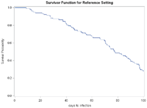
This SAS code produced the image shown in Figure 19.5, below, which is the survival probability curve for the entire sample of N=100 cases monitored over 150 days. Notice that there is an inflection point in the curve at 100 days. This inflection point corresponds to the censoring limit of 100 days and is shown more explicitly in Figure 19.6 where we change the command time days; to the command: time days * case(0);
Figure 19.5 Life Table Survival curve for all individuals in the data set
Figure 19.6 Life Table Survival curve with explicit right censoring at 100 days
Figure 19.6 above shows the survival probability for each event among the cases and holds the non-cases constant at a probability level of 0.3. Further, when we include the censoring criteria using the command: time days * case(0); a summary table indicating the number of cases that fail prior to the demarcation point (100 days) and the number of cases that exceed the demarcation point is also included, as shown here.
| Summary of the Number of Censored and Uncensored Values | |||
| Total | Failed | Censored | Percent Censored |
| 100 | 70 | 30 | 30.00 |
Next we include a command to show the differences in time to event with a grouping variable. Here we use the strata command to group the data by sex, while maintaining the influence of censoring at 100 days.
PROC LIFETEST METHOD=LIFE plots=(s)data=sample.zika notable;
time days * case(0) ;
strata sex;
format case casefmt. sex sexfmt. ;
The code produces a summary table of the number of males and females that failed or exceeded the demarcation point of 100 days and a graph of the survival probability curves for male and females.
| Summary of the Number of Censored and Uncensored Values | |||||
| Stratum | sex | Total | Failed | Censored | Percent Censored |
| 1 | female | 71 | 52 | 19 | 26.76 |
| 2 | male | 29 | 18 | 11 | 37.93 |
| Total | 100 | 70 | 30 | 30.00 |
Figure 19.7 Life Table Survival Curves With Explicit Right Censoring at 100 Days for Males and Females
In this next analysis we separate the data using strata=sport, while maintaining the right censoring of the data at 100 days. As shown in the approach used to separate the data by sex, this code produces a summary table of the number of individuals in each of the sport groups that failed or exceeded the demarcation point of 100 days as well as a graph of the survival probability curves for each sport.
| Summary of the Number of Censored and Uncensored Values | |||||
| Stratum | sport | Total | Failed | Censored | Percent Censored |
| 1 | equestrian | 22 | 15 | 7 | 31.82 |
| 2 | golf | 23 | 19 | 4 | 17.39 |
| 3 | gymnastics | 24 | 14 | 10 | 41.67 |
| 4 | swimming | 17 | 13 | 4 | 23.53 |
| 5 | track & field | 14 | 9 | 5 | 35.71 |
| Total | 100 | 70 | 30 | 30.00 |
Figure 19.8 Life Table Survival Curves With Explicit Right Censoring at 100 Days for Sport Groups
Part 3: The Kaplan-Meier Approach
The Kaplan-Meier approach to survival analysis differs slightly from the applications using METHOD=LIFE in the PROC LIFETEST procedure. When we use the METHOD=KM in the PROC LIFETEST procedure we generate a series of survival probability estimates referred to as the Kaplan-Meier estimates (heretofore referred to as the KM estimates), and corresponding survival probability curves for the KM estimates.
In the KM estimates values are given for the probability change each time an individual becomes a case up to the demarcation point of 100 days. This approach is more precise in reporting the time at event and does not summarize the data across an interval as is done with the METHOD=LIFE in the PROC LIFETEST procedure.
A comparison of the output from the METHOD=LIFE and the METHOD=KM is shown in the comparison of the tables up to the first 12 cases that became infected. Notice that the METHOD=LIFE approach summarizes the estimates within a set of intervals, while the METHOD=KM approach provides the continuous probability values for each individual within the cohort of interest.
Table 19.5 Survivor function for Zika virus using METHOD = LIFE in Proc Lifetest
| Days Interval | Abbreviated table showing results for The LIFETEST Procedure | ||||||||
| Lower interval | Upper interval | Number failed | Number censored | Effective sample size | Conditional probability of failure | Conditional probability of failure Standard error | Survival | Failure | Survival Standard error |
| 0 | 20 | 6 | 0 | 100.0 | 0.0600 | 0.0237 | 1.0000 | 0 | 0 |
| 20 | 40 | 12 | 0 | 94.0 | 0.1277 | 0.0344 | 0.9400 | 0.06 | 0.023 |
When we use the METHOD=KM approach in the PROC LIFETEST procedure the following estimates are generated. Note these estimates only refer to the first 12 cases designated as infected within the original data set of n=100 cases.
Table 19.6 Survivor function for Zika virus using METHOD = KM in Proc Lifetest
Abbreviated table showing results for The LIFETEST Procedure
| Days | Survival | Failure | Survival Standard Error | Number Failed |
Number Remaining |
| 0.000 | 1.0000 | 0 | 0 | 0 | 100 |
| 8.800 | 0.9900 | 0.0100 | 0.00995 | 1 | 99 |
| 11.780 | 0.9800 | 0.0200 | 0.0140 | 2 | 98 |
| 12.540 | 0.9700 | 0.0300 | 0.0171 | 3 | 97 |
| 12.800 | 0.9600 | 0.0400 | 0.0196 | 4 | 96 |
| 14.120 | 0.9500 | 0.0500 | 0.0218 | 5 | 95 |
| 15.860 | 0.9400 | 0.0600 | 0.0237 | 6 | 94 |
| 21.240 | 0.9300 | 0.0700 | 0.0255 | 7 | 93 |
| 22.560 | 0.9200 | 0.0800 | 0.0271 | 8 | 92 |
| 24.720 | 0.9100 | 0.0900 | 0.0286 | 9 | 91 |
| 27.280 | 0.9000 | 0.1000 | 0.0300 | 10 | 90 |
| 27.780 | . | . | . | 11 | 89 |
| 27.780 | 0.8800 | 0.1200 | 0.0325 | 12 | 88 |
The difference in the two methods is further exemplified in the comparison of the two survival curves shown in Figure 19.9. The survival curve for the METHOD=LIFE approach is a summary curve while the survival curve for the METHOD=KM approach shows more precise estimates of failures (individuals reporting infection) over the entire time interval. In both curves the data are right censored at days=100, and as such no survival probabilities are reported for individuals that have not become a case as of the 100 days demarcation point, in the data set.
| Survival probability curve using Method=LIFE in SAS Proc lifetest | Survival probability curve using Method=KM in SAS Proc lifetest |
Figure 19.9 Comparison of Survival Curves With Explicit Right Censoring for life-table analysis versus Kaplan-Meier estimation
Part 4: Comparing Kaplan-Meier Survival Estimates with Log Rank and Wilcoxon Tests
In the PROC LIFETEST procedure we can evaluate the difference between survival probability curves by computing two non-parametric tests: i) the Log Rank Test and ii) the Wilcoxon test. The tests are computed with the PROC LIFETEST procedure when including the strata command, as shown here:
PROC LIFETEST plots=(s) data=sample.zika2 ;
time days * case(0);
strata sex;
format case casefmt. sex sexfmt. ;
title ‘Kaplan Meier Estimates with log rank and Wilcoxon tests’;
label days =’days to infection’;
The strata command separates the computation of survival probabilities by different subgroups of the variable used in the strata command. In our Zika data set, survival probabilities are estimated for the males and females in the observed sample. The graphical illustration of the survival probability curves is shown in Figure 19.10 below and the statistical comparison of the survival curves is shown in the following two tests.
The Log-Rank test and the Wilcoxon test are two non-parametric tests that enable users to compare the survival probability curves based on Kaplan-Meier Survival Estimates for each subgroup within designated strata. The results for the comparison of the Survival Probability Curves for males versus females are shown here.
Table 19.7 Test to evaluate the survival curves
| Test | Chi-Square | DF | Pr > Chi square |
| Log-Rank | 2.8240 | 1 | 0.0929 |
| Wilcoxon | 4.2191 | 1 | 0.0400 |
The p value indicates that the difference in survival curves for males versus females was found to be significantly different at p<0.04 for the Wilcoxon test, while the difference was significant at p<0.09 when tested using the log-rank test. The overall conclusion from this test is that the curves for the two survival probabilities were different. However, it should be noted that the Log-Rank test is the more powerful of the two tests because it is based on the assumption that the proportional hazard rate is constant at each time point. This means that the likelihood for an individual to be infected (i.e. become a case) is constant across all time points for all individuals[3].
Figure 19.10 illustrates the survival probability curves for males versus females in our Zika dataset. These curves are based on the product-limit estimates (aka Kaplan-Meier estimates) for the survival probability series within each level of the strata. Notice that the two survival curves cross early in the recording. This cross over of KM curves corresponds to the p value identified with the Wilcoxon analysis. In the statistical comparison of survival curves a stronger Wilcoxon outcome is likely to occur when one of the comparison groups has a higher risk of demonstrating the time to the event (becoming a case) earlier in the recording, versus a higher risk of being infected later. The higher risk of being infected (i.e. failing, dying, becoming a case) corresponds with a higher number of days to the event which increases the likelihood of a significant log-rank test outcome if this is demonstrated by one group more than another.
Figure 19.10 Comparison of Survival Curves With Explicit Right Censoring for Kaplan-Meier estimation of males versus females
Part 5: Computing the Cox Proportional Hazard Regression Analysis
The data in a survival analysis can be used in a special type of regression procedure known as the proportional hazard model. This approach to using regression modeling was developed by Cox[4] and builds on the regression approaches that we have discussed earlier in this text.
In simple linear regression we can create equations in which a predictor variable, or set of predictor variables are used to explain the variance in an outcome variable (the dependent variable), as shown in the following simple linear regression and multiple regression equations.
A simple straight-line or linear regression equation:
where: is the dependent variable, is the slope element by which we adjust the predictor () variable, is the independent or predictor variable, and is the
– intercept (i.e. the point where the response graph crosses the vertical axis).
The simple linear regression equation in its most basic form helps us to understand the relationship between two variables, one designated as the and the other designated as the . Together these variables help us to predictor or explain an outcome, while adjusting for the variance between the two measures.
A multiple regression equation:
where: is the dependent variable, is the slope element by which we adjust the predictor () variable, is the independent or predictor variable, and is the
– intercept. In this equation, the subscript (i) is a counter for each of the predictor variables used in the equation.
The multiple linear regression equation is an expansion of the simple linear regression, and under a univariate model has one but two or more Again, the regression procedure helps us to predict or explain the outcome while adjusting for the variance in the predictor () variables. In multiple regression we can determine the slope of a predictor variable – the coefficient by which the variable is multiplied, while holding all other variables in the model constant. In this way we are able to determine the significance of each variable in the equation with respect to all of the variables in the equation.
In the Cox proportional hazard regression, also referred to as the Cox regression, the concepts of simple and multiple regression equations are the same, however the dependent variable is comprised not of a single scalar score, but rather of the hazard function representing the relationship between survival probability and time to an event.
As stated earlier, the hazard function provides an estimate of an event happening by a given time or within a given interval of time. The hazard function does not provide a probability estimate; therefore the estimate can exceed 1. Rather the hazard function indicates how likely an event is expected to occur by a given time.
In the computation of the Cox regression we develop a statistical regression model comprised of a dependent variable which consists of a hazard function and a set of independent variables which consist of predictors of the dependent variable, all based on a time based distribution referred to as the Weibull distribution. The Weibull distribution is familiar to the field of engineering because it is helpful in describing reliability and failure of a measured device over time. The applicable characteristic of the Weibull distribution for survival analysis is that it provides a mathematical foundation for failure rate throughout the lifetime of a measurement period. In the Weibull distribution the failure rate is shown to decrease with time reaching a plateau that is relatively constant[5]. The Weibull distribution fits applications for survival analysis since higher failure rates (i.e. time to an event) occur more often prior to the censoring demarcation point as shown in Figure 19.11.
Figure 19.11 Schematic of a Weibull distribution
As in the application of simple and multiple linear regression procedures, in the application of the Cox regression the user can establish regression coefficients for each of the predictors of the dependent variable to determine the magnitude and direction of the predictor acting on the dependent variable.
In our Zika virus example, we use Cox regression to determine the risk of infection based on the ratio of the probability density function and survival probabilities for time to infection as the dependent variable, and individual’s sex and sport as predictor variables.
In other words, using the simulated dataset for the Olympic athletes and Cox regression we can evaluate the likelihood of being infected with Zika virus based on whether the individual was male or female, and the type of Olympic sport in which they were participating.
In the following sample code we use the proc phreg; procedure to produce output for the Cox Proportional Hazard Function. However, it is good practice to explain the overall model that we are testing. Here our hazard function is based on the number of days to infection, and the covariates are sex and sport type, along with the interaction of sex by sport type.
proc phreg plots=survival;
class sex sport;
model days*case(0) = sex sport sex_sport;
title ‘Cox Proportional Hazard Analysis for Zika Virus by sex and sport’;
label days =’days to infection’;
The output shown below provides a graphic image of the survival curve and associated tables representing the statistical analyses.
Plot of the survival probability curve from proc phreg
The summary table of the number of cases that exceeded the censoring demarcation point is presented in Table 19.8 below. The results indicate that 30 of the 100 simulated cases.
Table of Proportion of Censored Observations from the Survival Curves
| Summary of the Number of Event and Censored Values | |||
| Total | Event | Censored | Percent Censored |
| 100 | 70 | 30 | 30.00 |
Next, the model fit statistics are presented followed by the test of the null hypothesis that the predictor variables as greater than 0. The model fit statistics are most often used when comparing more than one model, in which case we evaluate the AIC criteria to select the lowest value as suggesting a more appropriate fitting model. In the example shown here, this output is less relevant as we on have one model to consider. The column representing With Covariates is important to consider as it indicates that as we add predictor variables to the equation we decrease the criteria value, whereby lower values are considered to represent a better fit.
Table of a Model Fit Statistics for the Application of the Cox PHREG
| Model Fit Statistics | ||
| Criterion | Without Covariates |
With Covariates |
| -2 LOG L | 578.185 | 569.236 |
| AIC | 578.185 | 581.236 |
| SBC | 578.185 | 594.727 |
The main outputs for us to consider from the application of the proc phreg; procedure for this example are the tables of test for Global Null Hypothesis: Beta=0 and the Analysis of the Maximum Likelihood, shown below. The test of the Global Null Hypothesis: Beta=0 is suggesting that the predictor variables do not have an effect on the calculated value of the hazard function.
Table of Tests of Beta=0 for the Application of the Cox PHREG
| Testing Global Null Hypothesis: BETA=0 | |||
| Test | Chi-Square | DF | Pr > ChiSq |
| Likelihood Ratio | 8.9485 | 6 | 0.1765 |
| Score | 9.8384 | 6 | 0.1316 |
| Wald | 9.3857 | 6 | 0.1530 |
The results presented in the table above for the test of the Global Null Hypothesis: Beta=0 illustrate the results of three tests of the null hypothesis: i) the likelihood ratio test, ii) the Score test, and iii) the Wald test. Notice that the probability estimates for each Chi-square test are similar in that none of the p values supported a significant difference between the predictor variables and 0.
Since the predictor variables included the example were discrete class variables (no continuous covariates were included in the model), we also included the class sex sport; statement in the proc phreg; procedure. The output generated a table of the Type 3 tests (also referred to as Joint tests) to determine if each of the categorical discrete variables were significantly different than 0. The results of the Wald Chi-square statistic indicate that there was no significant effect of any of the categorical variables on the computed hazard function for the days to infection from the Zika virus.
Table of Type 3 Tests from Proc PHREG
| Type 3 Tests | |||
| Effect | DF | Wald Chi-Square | Pr > ChiSq |
| sex | 1 | 0.5229 | 0.4696 |
| sport | 4 | 1.3533 | 0.8523 |
| sex_sport | 1 | 0.0311 | 0.8601 |
The maximum likelihood estimates produced by the SAS proc phreg enable us to provide the parameter estimates that correspond to the predictor variables included in the regression equation. The underlying algebraic regression equation[6] for the Cox Proportional Hazard Model is given as:
[latex]h(t) = h_0 (t)exp(x\beta_{x})[/latex]
Therefore, the parameter estimates refer to the coefficients for each predictor variable in the equation.
Maximum Likelihood Estimates from PROC PHREG
| Parameter | DF | Parameter Estimate |
Standard Error |
Chi-Square | Pr > ChiSq | Hazard Ratio |
Label | |
| sex | 1 | 1 | -0.49114 | 0.67917 | 0.5229 | 0.4696 | 0.612 | sex 1 |
| sport | 1 | 1 | 0.47592 | 1.51352 | 0.0989 | 0.7532 | 1.609 | sport 1 |
| sport | 2 | 1 | 0.00554 | 1.11315 | 0.0000 | 0.9960 | 1.006 | sport 2 |
| sport | 3 | 1 | 0.13256 | 0.80301 | 0.0273 | 0.8689 | 1.142 | sport 3 |
| sport | 4 | 1 | -0.13920 | 0.52854 | 0.0694 | 0.7923 | 0.870 | sport 4 |
| sex_sport | 1 | -0.03689 | 0.20926 | 0.0311 | 0.8601 | 0.964 |
The results presented in the table above indicate that none of the predictor variables produced a significant parameter estimate, therefore we can conclude that the days to infection were not different by gender nor the sport in which the athlete participated.
[1] Wicklin, R. (2011) http://blogs.sas.com/content/iml/2011/10/19/four-essential-functions-for-statistical-programmers.html
[2] Introduction to Survival Analysis in SAS.UCLA: Statistical Consulting Group.From http://www.ats.ucla.edu/stat/sas/seminars/sas_survival/ (accessed Feb 20, 2017)
[3] Bewick, V., Cheek, L., Ball, J., Statistics review 12: Survival analysis, Critical Care 2004, 8:389-394.
[4] The Cox Proportional Hazard regression is based on Sir David Cox 1972 paper: Regression Models and Life-Tables (1972), J. R. Stat. Soc. B, 34:187–220).
[5] The weibull.com reliability engineering resource website is a service of ReliaSoft Corporation.
Copyright © 1992 – 2017 ReliaSoft Corporation. All Rights Reserved.
[6] Introduction to Survival Analysis in SAS.UCLA: Statistical Consulting Group.From http://www.ats.ucla.edu/stat/sas/seminars/sas_survival/ (accessed Feb 20, 2017)
