
Measuring Correlation, Association, Reliability and Validity
38 Measures of Association – Part I: The McNemar Chi-Square
Part 1: The McNemar Test of Symmetry[1]
This chapter is presented in 2 parts. In the first part, we explore the McNemar Chi-Square Test of Symmetry, where the notion of symmetry is based on the 2 x 2 chi-square comparing elements on the diagonal axis from top left to bottom right, against the off-diagonal elements from bottom left to top-right. In the second part, we explore the question, if we do not observe a significant difference between two measures based on the calculations of the McNemar Chi-Square test, then should we expect that there is an implicit association between the two measures?
Building on the concept of association between independently measured outcome variables, the 2 x 2 table can also be used to organize our data so that we can test the association between the outcome on one variable against the outcome on another variable.
Field testing, whereby we collect data in real-world research applications to evaluate constructs that we would normally see in laboratory tests are often used in health research to evaluate community-based samples. In health research, there are several opportunities to compare field test variables against suggested gold standard variables to determine how closely the field test outcomes match that which we would expect to observe from more controlled laboratory measures.
For example, in measuring the fitness levels within a community, it may not be practical to have every person in the community perform a laboratory-based treadmill exercise test that would evaluate the precise level of maximal oxygen consumption — a measure of cardiorespiratory fitness capacity (VO2 max ml/kg min). Rather, we can simply recruit a sample of individuals and ask them to perform a one-mile walk test using a planned procedure in which we confirm the distance travelled and the time taken to walk the distance. Combining this information with their height, weight and heart rate response while performing the walk will provide reliable evidence to accurately predict the individual’s oxygen consumption capacity – their VO2 max (ml/kg min).
The one-mile walk test is considered to be an efficient field test to provide accurate predictions of an individual’s oxygen consumption capacity because the outcomes on such a test have been compared to laboratory estimates of VO2 max (ml/kg min) and verified by several independent researchers. A simple way to test the notion of an association between a field test and a laboratory test is to have a group of individuals complete both tests and then measure the relationship between the combined outcome measures. That is, to organize the data as pairs of outcomes and then determine the ratio of the number of concordant or expected pairs against the number of discordant pairs.
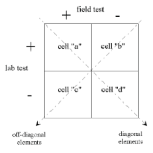
In the application of the McNemar Chi-Square test, use the following diagram to organize the association between a given field test response and a corresponding laboratory test response. The organization of these outcomes provides the data that are used to calculate the chi-square statistic (based on a 2 x 2 design).
The diagram presents a box with four cells labelled “a”, “b”, “c”, and “d”. The top margin of the box is labelled field test (+, -), while the left margin is labelled laboratory test (+,-). In order for a participant’s response to be placed in the “a” cell, the paired outcome of their scores on the field and laboratory test would be (+) on BOTH tests. Likewise, for a participant’s response to be placed in the “d” cell, the paired outcome of their scores on the field and laboratory test would be (-) on BOTH tests. The “a” and “d” cells represent the concordant pairs.
Similarly, for a participant’s response to be placed in the “b” cell, the paired outcome of their scores would be (+) on the laboratory test and (-) on the field test. Finally, for a participant’s response to be placed in the “c” cell, the paired outcome of their scores would be (-) on the laboratory test and (+) on the field test. The “b” and “c” cells represent the concordant pairs.
Using this design and the McNemar Chi-Square statistic, the researcher can evaluate the concordant pairs (the diagonal elements) while adjusting for the discordant pairs (the off-diagonal elements).
Figure 1: Design for the Application of the McNemar Chi-square Statistic
It is important to note that there are two specific preparatory steps to be considered before applying the McNemar Chi-square to test the association between two independent tests.
- First, the two tests, which in this example will produce a field test response and a laboratory test response, must be organized to demonstrate pair-wise data. That is, the same individual (or a matched pair of individuals) performs both the laboratory test and the field test.
- Second, regardless of the initial variable type, the results for each test are transformed into a binary score. This can be done by splitting the array of data for each test at the median (middle) score and establishing the polarity of the top and bottom halves of the array. In order to arrange the data in this way, simply list the scores from highest to lowest (or lowest to highest) and split the list (the array) at the mid-point (median score) on the list. All scores above the median score are labelled (+) and all scores below the median (-) are labelled negative. when we arrange the outcomes of scores as matched pairs we can distribute the outcomes in the 2 x 2 design relative to the combined response on the two tests.
The following abbreviated data table presents the cell outcomes for a set of data based on a sample size of 86 participants organized to meet the criteria stated above. Notice that each individual completed both the laboratory (Column 2) and field-test (Column 4) and therefore has a VO2 max score on each test. The median scores for each variable (median score on the laboratory test = 44 (Column 3) , and median score on the field test = 37 (Column 35)) were identified and the individual’s response in relation to the respective median scores was noted.
Next, the 2 x 2 cell membership was established for each participant in relation to the design shown in Figure 1, above. That is, the cell assignment in the 2 x 2 table for each participant based on whether they scored above or below the median score on both variables is indicated with “+” for scores at or above median score, and “-” for scores below the median score (Column 6).
Table of Raw data used in the McNemar Chi-Square Test of Symmetry
|
Participant ID (Column 1) |
Score on laboratory test: The Treadmill test (Column 2) | Score in relation to treadmill median score => 44
(Column 3) |
Score on field test: One-mile walk test (Column 4) | Score in relation to one mile walk median score => 37
(Column 5) |
2 x 2 cell membership
(Column 6) |
| 001 | 54 | + | 45 | + | + + (cell a) |
| 002 | 25 | – | 23 | – | – – (cell d) |
| 003 | 46 | + | 33 | – | + – (cell b) |
| 004 | 42 | – | 38 | + | – + (cell c) |
| 005 | 40 | – | 40 | + | – + (cell c) |
| … | … | … | … | … | … |
| 084 | 29 | – | 30 | – | – – (cell d) |
| 085 | 47 | + | 28 | – | + – (cell b) |
| 086 | 71 | + | 72 | + | + + (cell a) |
The membership for pairs of outcomes is presented in (Column 6) of the chart above. Using the median score within each variable enabled the separation of the group into one of four outcomes, based on the variable’s median reference value. The data used to identify membership is binary for each variable.
Further, while cells a and d are important in that they provide the number of concordant pairs, the McNemar Chi-square is actually a test of symmetry used to determine the significance of the number of discordant pairs – the off-diagonal elements.
Simply put, The McNemar procedure tests the equality of frequencies in pairs of cells that are symmetric around the diagonal of a 2 by 2 design (the diagonal elements are the paired data in the upper-left cell: cell “a”, and lower right cell: cell “d”). In the computation of the McNemar equivalence estimates, the frequencies in the major diagonal (upper left cell to lower right cell) are ignored. The null hypothesis (Ho: p1. = p.1) which is that the row 1 probability = the column 1 probability, and implies that the proportion of individuals who score high on the laboratory test and low on the field test will match the proportion of individuals who score high on the field test and low on the laboratory test.
The outcome data for a sample of 86 individuals that completed both tests are presented in Table 2 below.
Table 2. Observed pairwise counts for laboratory and field test measures arranged for the McNemar Chi-square test
| Laboratory test (+) | Cell a =23 | cell b =12 | [latex]p_{1.} = {(a+b)\over{N}}[/latex]
[latex]p_{1.} = 0.41[/latex] |
| Laboratory test (-) | cell c = 19 | cell d = 32 | [latex]p_{2.} = {(c+d)\over{N}}[/latex]
[latex]p_{2.} = 0..59[/latex] |
| N=86 | Field test (+) | Field test (-) | Row Probabilities |
Once we organize the observed data according to the appropriate cell membership we can write the following SAS program to estimate the chi-square observed value
SAS Program to Compute the McNemar Chi-Square Statistic
DATA MCNKAP;
TITLE ‘MCNEMAR AND KAPPA STATISTICS’;
INPUT ROW COL OUTCOME;
DATALINES;
1 1 23
1 2 12
2 1 19
2 2 32
;
PROC SORT DATA=MCNKAP; BY ROW COL;
PROC FREQ;
TABLES ROW*COL /AGREE;
WEIGHT OUTCOME;
RUN;
Again, as in the previous applications of the 2 x 2 test, we can evaluate the chi-square observed score against the chi-square critical score of 3.84. The chi-square critical value is the expected chi-square statistic for a 2 x 2 table with a degrees of freedom (row-1) x (column -1) = 1 and an alpha level or probability level of p < 0.05.
The McNemar Test is used to test the relationship between the matched pairs of data on the two variables in the 2 x 2 table. That is we are interested in the proportion of responses in the cells related to the marginal variables (i.e. the row variable – the lab test with the column variable – the field test). Specifically, the null hypothesis is testing the following comparison of proportions s that the row 1 probability = the column 1 probability l. Which can also be written as: [latex]H_0 : p_{1.} =p_{.1}[/latex]
The results of the SAS computation of the McNemar Chi-Square are shown in the table below.
McNemar Chi-square test for pairwise counts of laboratory and field test measures
| McNemar’s Test | |
| Statistic (S) | 1.5806 |
| DF | 1 |
| Pr > S | 0.2087 |
Since the chi-square observed value in this sample computation is 1.59 with a probability of 0.21 then we accept the null hypothesis of no difference between the field test and the laboratory test.
The Stepwise formula to compute the McNemar Chi-Square statistic is shown here:
| 1. [latex]z_{1}={(n_{12} - n_{21})\over{\sqrt(n_{12} + n_{21})}}[/latex] | where: [latex]n_{12} = \textit{cell b as in } row_{1}, column_{2}[/latex] and [latex]n_{21} = \textit{cell c as in } row_{2}, column_{1}[/latex] |
|
| 2. [latex]z_{1}={(12- 19)\over{\sqrt(12 + 19)}}[/latex] | 3. [latex]z_{1}={(-7)\over{\sqrt(31)}}[/latex] | 4. [latex]z_{1}= -1.26[/latex] |
To calculate the McNemar chi-square statistic from a z-score, simply square the z-score.
The McNema Statistic can be shown as a Z score =-1.26 or as a [latex]{\chi}^2 = 1.58[/latex]
If the McNemar estimate is presented as a Z score then we compare the value against -1.96 to +1.96, as the region of accepting the null hypothesis. Likewise, if the McNemar estimate is presented as a [latex]{\chi^2}[/latex] then we compare the value against 3.84, where [latex]{\chi^2}[/latex] scores < 3.84 are included in the region of accepting the null hypothesis (area under the normal curve) shown below.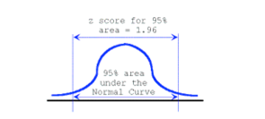
NOTE: A webulator to calculate the McNemar and Kappa Statistics is presented in the chapter after next, and is currently available at: https://health.ahs.upei.ca/webulators/test_mcnKap.php
[1] This section is based on the following published work: Montelpare, W.J., and McPherson M., (2000) Client-side processing on the InterNet: Computing the McNemar test of symmetry and the kappa statistic for paired response data. The International Electronic Journal for Health Education, 3(3): 253-271.
