
Goodness of Fit and Related Chi-Square Tests
18 Multi-way Contingency Table Chi-Square Analysis
Application of the Goodness of Fit Chi-square analysis to multi-way tables (3×3 and beyond)
Another form of the chi-square goodness of fit test is shown in the analysis of multi-way contingency tables. In the following example we show the use of a 3 x 3 contingency table to evaluate the association between visits to the emergency room in a cohort of COPD patients and the use of an online wellness program designed to provide customized programming for COPD patients.
In the following study a group of COPD patients were taught how to use an online program designed to provide up to date information about nutrition, exercise, stress and medications that could prevent the exacerbation of a dyspnea[1] response by the patient. The data were presented in several formats and included both direct and indirect communications between healthcare providers and the patients. The researchers organized the following contingency table to test the association between use of the online tools and visits to the emergency department in an 18-month period.
Table 18.1 Raw Data used to Evaluate the Association Between the Use of Online Tools and Visits to the Emergency Department
| N= 375 | 0 Visits to the emergency department | 1-3 Visits to the emergency department | > 3 Visits to the emergency department |
|---|---|---|---|
| Infrequent use of the online tools: less than once per week | 12 | 55 | 100 |
| Occasional use of the online tools: 1-3 times per week |
21 | 37 | 19 |
| Frequent use of the online tools: 4 or more uses per week | 105 | 11 | 15 |
| Column Totals | 138 | 103 | 134 |
We can use the webulator presented below to compute the chi-square statistic for the multi-way (3 x 3 ) contingency table . Note that the equation for the 3 x 3 contingency table is the same as all chi-square tables.
[latex]{\chi}^2 = \sum\frac{(obs - exp)^2}{expected}[/latex]
In the data processing panels shown here the row and column sums (Panel 1) are used to compute the expected frequencies for each cell (Panel 2). The third panel provides the actual chi-square test. The sum of the variance computations is the chi-square statistic.
The computed score is referred to as the chi-square observed. After computing the chi-square for the observed scores we next determine the chi-square critical score which represents the chi-square for the expected population. The chi-square critical score for a three by three frequency table is determined by computing the “degrees of freedom” for our response set.
The computation of the degrees of freedom is as follows:
degrees of freedom = (number of rows – 1) x (number of columns -1)
degrees of freedom = (3-1) x (3-1)
degrees of freedom = (2) x (2)
degrees of freedom = 4
and the “chi-square critical value” for degrees of freedom of “4” at p<0.05 = 9.49
Our null hypothesis in this scenario is that there is no association between the row and column variables.
If the “chi-square observed value” is › the “chi-square critical value of 9.49” then we would reject the null hypothesis and state that there is an association between the row and column variables. However, if the “chi-square observed value ” is ‹ the “chi-square critical value of 9.49”, we would ACCEPT the null hypothesis and state that the distributions ARE EQUAL.
The results of our analysis show that there is a relationship between the use of online tools and visits to the emergency room. That is, individuals that had a lower frequency of use of online tools were more likely to visit the emergency room than individuals that were considered frequent users of the online tools.
SAS Code used to demonstrate the computation of the 3 x 3 Chi-Square Goodness of Fit
In the example above we computed the differences in visits to the hospital by individuals that used (or chose not to use) online wellness resources. The following is the SAS code applied to the computations above. The study intended to compare the three distributions of hospital visits among online health resource users (or non-users).
The data set was comprised of three variables: Frequency of online health resource use: where 1 = ‘infrequent’, 2 = ‘occasional’, 3 = ‘frequent’;
The category of the number of visits to the hospital: 1 = ‘0 visits’, 2 = ‘1 to 3 visits’; and a third variable which was the number of cases reported to visit. The relevant SAS code used to process this two-group chi-square goodness of fit is shown here:
PROC FORMAT;
VALUE USEFMT 1 = ‘INFREQUENT’ 2 = ‘OCCASIONAL’ 3 = ‘FREQUENT’;
VALUE VISITFMT 1 = ‘0 VISITS’ 2 = ‘1 TO 3 VISITS’. 3 = ‘> 3 VISITS’;
DATA CHIVISIT;
TITLE ‘ON LINE WELLNESS TOOLS REDUCE HOSPITAL VISITS’;
INPUT TOOLS VISITS NCASES @@;
LABEL NCASES = ‘NUMBER OF HOSPITAL VISITS REPORTED’
VISITS = ‘CATEGORIES FOR VISITS’
TOOLS = ‘FREQUENCY OF ONLINE RESOURCE USE’;
DATALINES;
1 1 12 1 2 55 1 3 100 2 1 21 2 2 37 2 3 19
3 1 105 3 2 11 3 3 15
;
PROC SORT DATA= CHIVISIT; BY VISITS;
PROC GCHART;
BLOCK TOOLS /SUMVAR=NCASES GROUP=VISITS NOHEADER DISCRETE COUTLINE=RED WOUTLINE=1 ;
FORMAT TOOLS USEFMT. VISITS VISITFMT. ;
TITLE1 ‘HOSPITAL VISITS BY USE OF ONLINE HEALTH RESOURCES’;
PATTERN1 COLOR = LIGHTBLUE;
PROC FREQ;
TABLES TOOLS*VISITS / CHISQ ; WEIGHT NCASES;
FORMAT TOOLS USEFMT. VISITS VISITFMT. ;
TITLE ‘NUMBER OF HOSPITAL VISITS REPORTED’;
TITLE2 ‘TWO SAMPLE GOODNESS OF FIT STUDY’;
The SAS code above produced the following block chart of the distribution of the visits to the hospital related to the use of online resources.
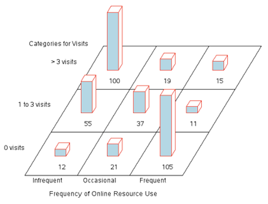 Graph 18.1 Distribution of visits to the hospital related to the use of online resources
Below is the tabular output for the PROC FREQ procedure to produce the frequency distribution of the visits to the hospital by the use of online resources. The data represent a two-sample goodness of fit study design.
|
|
||||||||||||||||||||||||||||||||||||||
|---|---|---|---|---|---|---|---|---|---|---|---|---|---|---|---|---|---|---|---|---|---|---|---|---|---|---|---|---|---|---|---|---|---|---|---|---|---|---|---|
The following is a summary table generated by the PROC FREQ procedure. Here we can review the chi-square statistic and its corresponding p-value, and compare the value produced by SAS ([latex]{/chi^2}= 191.15 p0.001[/latex] to that which we produced above with our Webulator (also ([latex]{/chi^2}= 191.15 p0.001[/latex] ). Note, the sample size is provided at the end of the SAS output: Sample Size = 375.
| Statistic | DF | Value | Prob |
| Chi-Square | 4 | 191.1463 | <.0001 |
| Likelihood Ratio Chi-Square | 4 | 202.0115 | <.0001 |
| Mantel-Haenszel Chi-Square | 1 | 148.5705 | <.0001 |
| Phi Coefficient | 0.7139 | ||
| Contingency Coefficient | 0.5811 | ||
| Cramer’s V | 0.5048 |
[1] Dyspnea is a sensation, referring to the sensation of shortness of breath or the feeling of having difficulty breathing.
