In the following example, we consider the goodness of fit chi-square test with five response categories.
The biweekly lottery – Lotto 649 provides players with an opportunity to win millions of dollars if they can select the set of six numbers that are randomly drawn from the set of numbers from 1 to 49. Since the lottery is purported to be random, the chance associated with a player’s single ticket matching the six numbers drawn at random is based on the combinatorial formula for 49 choose 6 and has a probability of 1 ÷ 49C6.
The probability associated with every single ticket is the same and is 1 in 13,983,816 possible combinations of 6 numbers. So then, what if we wanted to test the randomness of this lottery? In the following example, we will use the chi-square goodness of fit test to determine if each number is random with respect to selection, and that there is no apriori pattern of numbers from one range or another within the set of 49 occurring more frequently or with a systematic selection pattern.
To begin we need to organize the range of possible outcomes into manageable categories that can be processed with the chi-square goodness of fit test. Given that the range of all possible outcomes for the lotto is from 1 to 49, we can organize the potential sampling space (1 to 49) into 5 categories as follows 1-9, 10-19, 20-29, 30-39, 40-49.
Further, if we wanted to test randomness, then we would need to sample more than one single week of numbers, so considering that there are 104 draws per year we could use an entire year’s worth of data to establish the frequency distribution of numbers drawn, and after organizing the outcomes into the 5 categories determine the chi-square goodness of fit, statistically.
Step 1: after establishing that there are 5 categories for the outcome frequency distribution we would expect that the distribution or organization of the responses should be equal across all of the possible responses categories as follows:
Data represent the actual numbers that are drawn in a single year for the lotto 649. That is, in any given year there are 104 draws, which is based on 2 draws per week for 52 weeks. Therefore, in the lotto 649 example we have 624 possible numbers drawn à (2 draws per week for 52 weeks = 6 numbers x 104). These data can then be organized into the following 5 categories to represent the set of all possible numbers drawn in the one year so that a frequency distribution chart of the responses might look like this:
| 1 – 9 |
124 numbers |
| 10 – 19 |
125 numbers |
| 20 – 29 |
125 numbers |
| 30 – 39 |
125 numbers |
| 40 – 49 |
125 numbers |
Therefore, we can say from this chart that our responses to the research question should be evenly distributed across all of the possible responses.
Such a response pattern is consistent with our expected distribution. In other words, in an unbiased research study, we should expect that all possible responses are equally as likely to occur. We call this the unbiased null hypothesis, and state this in terms of frequencies of responses which are represented as f(k) = and is shown as follows:
H0: f1 = f2 = f3 = f4 = f5
Therefore, based on the null hypothesis, considering that each response category should have an equal number of responses, the formula to compute the expected responses might be as follows:
Now then let’s consider the following example. We asked students to generate 52 weeks of biweekly draws of the lotto 649 and then to sort the data so that we could simulate a test of the outcome distribution to determine how random the simulated lottery is at selecting numbers. The response options for the data produced for my 104 draws are given in the following table.
| 1-9 |
146 |
| 10-19 |
155 |
| 20-29 |
282 |
| 30-39 |
12 |
| 40-49 |
29 |
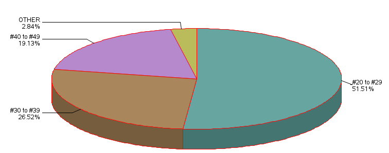
From this data, it would appear that a large proportion of the scores were found in the 20-29 range and only a few scores were found in the 30-39 range 283 of 624 or 28.5%. However, the lowest proportions of the scores (choices drawn) 12 of 624 = 1.9%
The chi-square test is, therefore, a useful statistical test to determine if the overall distribution of the responses in the observed sample is similar to or matches the expected distribution of responses in the target population (the “target population” being defined as all scores drawn) in this one year of simulated data.. The equation below is the basic equation for the goodness of fit chi-square test.
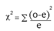
The equation shown here measures how closely an observed set of responses (the “ o” for “observed”) matches an expected set of responses (the “e” for “expected”).
So then how do we calculate the items that we use in the chi-square equation?
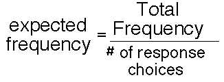
The observed frequencies are simply taken from the data recording sheet, but the expected frequencies are computed from the following formula:
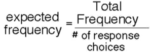
Another way to view the computation of the expected frequencies is to consider the null hypothesis which stated that:
H0: f1 = f2 = f3 = f4 = f5
and multiply the total frequency by the probability associated with each category, as in the following computations.
624 x 0.20 = 124.8
The chi-square is then used to compute whether or not the observed distribution fits a hypothetical or expected distribution. This can be accomplished by applying the formula to each row of the response table. The computation of the first row is shown here:

| Response Category |
Observed Frequency |
Expected Frequency |
(Obs – Exp)2 ÷ Exp |
| 1 – 9 |
146 |
124.8 |
3.60 |
| 10 – 19 |
155 |
124.8 |
7.31 |
| 20 – 29 |
282 |
124.8 |
198.01 |
| 30 – 39 |
12 |
124.8 |
101.95 |
| 40 – 49 |
29 |
124.8 |
73.54 |
In the calculation of the chi-square we see that in each row of the table, the observed score from the sample is subtracted from the expected score that represents the scores of the population. For example in ROW_1 of the table the observed score of 146 is subtracted from the expected score of 124.8. The difference of 21.2 is squared and the outcome is divided by 124.8, and the resulting value is 3.6. The calculation is repeated for each row of the table and the outcomes are added together to produce the chi-square value as shown below.
| Response Category |
Observed Frequency |
Expected Frequency |
(Obs – Exp)2 ÷ Exp |
|
3.60
+ 7.31
+ 198.01
+ 101.95
+ 73.54
384.41 |
Our next step is then to determine if the chi-square observed value is greater than the chi-square critical value, so that we can make a decision about the significance of the observed distribution.
The computed score is referred to as the chi-square observed. After computing the chi-square observed value, determine the chi-square critical score from a table of chi square values. The chi-square critical score represents what we should expect to observe for a distribution with five responses. The critical value is determined by computing the degrees of freedom for our response set.
The computation of the degrees of freedom is:
degrees of freedom = k possible responses -1
degrees of freedom = 5-1
degrees of freedom = 4
and the chi-square critical value for degrees of freedom of 4 at p<0.05 = 9.49
If the chi-square observed value is GREATER THAN the chi-square critical value of 9.49, we must reject the null hypothesis and state that the distribution of responses across the four categories IS NOT EQUAL. A large chi-square value, that is a value which exceeds the chi-square critical value demonstrates that the outcome is less likely to occur by chance.
Using the degrees for freedom for a one-sample chi-square, our degrees of freedom are:
degrees of freedom = “k” possible responses -1
degrees of freedom = 5-1
degrees of freedom = 4
and the “ chi-square critical value” for degrees of freedom of “4” is 9.49
Therefore, because our chi-square observed value of 384.41 is › the chi-square critical value of 9.49, we must reject the null hypothesis and state that the distribution of responses across the four categories IS NOT EQUAL.
We can check our calculations with the following SAS Program. This program produces a frequency distribution with chi-square analysis to evaluate the null hypothesis (see above), as well as a pie chart to show the proportion of times a number from each category was drawn in the lotto.
PROC FORMAT;
VALUE SLICE 1=’#1 to #9′ 2=’#10 to #19′ 3=’#20 to #29′
4=’#30 to #39′ 5=’#40 to #49′;
DATA GFIT_2;
INPUT LOTTOGRP N_DRAWS;
/* DEFINE THE AXIS CHARACTERISTICS */
AXIS1 LABEL=(“LOTTO CATEGORIES”)
VALUE=(JUSTIFY=CENTER);
AXIS2 LABEL=(ANGLE=90 “N TIMES CATEGORY VALUE DRAWN”)
ORDER=(0 TO 1000 BY 100)
MINOR=(N=3);
AXIS3 LABEL=(ANGLE=90 “LOTTO CATEGORIES”);
AXIS4 LABEL=(“N TIMES CATEGORY VALUE DRAWN”) ;
DATALINES;
1 146
2 155
3 282
4 12
5 29
;
/* HERE WE USE THE OPTION SUMVAR TO GRAPH THE SUM OF THE FREQ */
PROC FREQ ORDER=DATA; TABLES LOTTOGRP/CHISQ CL CELLCHI2;
WEIGHT N_DRAWS;
FORMAT LOTTOGRP SLICE. ;
TITLE ‘FREQUENCY DISTRIBUTION FOR N TIMES CATEGORY VALUE WAS DRAWN’;
TITLE2 ‘ONE SAMPLE GOODNESS OF FIT EXAMPLE K=5’;
RUN;
PROC GCHART DATA=GFIT_1;
PIE3D LOTTOGRP/SUMVAR=N_DRAWS TYPE=SUM DISCRETE PERCENT=ARROW
COUTLINE=RED WOUTLINE=1 FILL=solid SLICE = arrow clockwise
noLEGEND noheading value=none;
FORMAT LOTTOGRP SLICE. ;
TITLE1 ‘PIE CHART FOR N TIMES CATEGORY VALUE WAS DRAWN’;
PATTERN1 COLOR = LIGHTBLUE;
Run;
The output for the frequency distribution with corresponding chi-square is shown here:
| 146 |
23.40 |
146 |
23.40 |
| 155 |
24.84 |
301 |
48.24 |
| 282 |
45.19 |
583 |
93.43 |
| 12 |
1.92 |
595 |
95.35 |
| 29 |
4.65 |
624 |
100.00 |
The pie chart for the number of times a value was drawn within each category, expressed as a percent is shown here.
Webulator Form 1:
The following is a Goodness of Fit Webulator for k= 5 responses In the example above our raw data values for the cumulative times that a number was drawn from each category of the Lotto is shown here:
Distribution of Draws per Category
| 146 |
| 155 |
| 282 |
| 12 |
| #40 to #49 |
29
|
Enter these data into the webulator below for each of your category options and then click the button labeled CLICK ME. This will produce the sum of the five values that you entered and compute the expected frequency for the values in the table.
The important value from this Webulator is the computed chi-square score. The computed score is referred to as the chi-square observed. After computing the chi-square observed value, determine the chi-square critical score from a table of chi-square values. The chi-square critical score represents what we should expect to observe for the distribution with “k” responses. The critical value is determined by computing the “degrees of freedom” for our response set.
The computation of the degrees of freedom is: degrees of freedom = “k” possible responses -1
degrees of freedom = 4-1 –> degrees of freedom = 3
and the “chi-square critical value” for degrees of freedom of “3” at p<0.05 = 7.815
If the “chi-square observed value ” is › the “chi-square critical value of 7.815”, we must reject the null hypothesis and state that the distribution of responses across the response categories IS NOT EQUAL.
If you would you like to use the Webulators for your own applications, without this text visit: https://health.ahs.upei.ca/webulators/w_menu.php

