
Parametric Statistics
28 Estimating Confidence Intervals for a Sample Mean
Putting it all together
In research, we often collect information from a collection of individuals that are drawn from a larger group. Since the procedures for information collection have real costs, researchers are forced to make the assumption that the individuals selected for study are a true representation of all of the individuals within the larger group. In quantitative analyses the larger group is the population, (represented by the letter ‘N’), and the selected subgroup is referred to as the sample (represented by the letter ‘n’). Given the assumption that the sample represents the population from which it was drawn, then it is also assumed that any computations, estimates, or inferences based on the measures from the sample, must also represent the population from which the sample was selected.
As such, the average score computed for the sample is assumed to represent the average score for the population. Likewise, the variability of scores within the sample (the subgroup) is expected to represent the variability of the scores within the population (the larger group). Similarly, the standardized estimate of the differences computed for the sample should represent the standardized estimate of differences computed for the population.
The confidence interval is based on the following relationship between the sample means and the true population mean or [µ]:
the lower limit of the sample mean < µ < upper limit of the sample mean
This sentence is read as: The lower limit of the sample mean is less than the true population estimate which is less than the upper limit of the sample mean. Therefore: the population mean = sample mean ± sampling error : µ = [latex]\overline{x}[/latex] ± (SE),
where:
- µ refers to the measure of central tendency for the population
- is the sample mean and refers to the measure of centrality in a sample
- Standard Error (SE) — error due to randomness
There are two basic assumptions in this approach:
First, we assume that the sample mean is only our best estimate of the true population mean.
Second, we assume that the chance associated with the sample mean’s ability to represent the true population mean is dependent upon the ability of the sample scores to represent the population scores.
So that by adding or subtracting the sampling error to or from the sample mean we will be able to identify the range within which the true population estimate falls.
Standard Error
The term sampling error, which is also called the standard error of the mean, is a measure of the extent to which the sample means can be expected to vary due to chance. In other words, the standard error of the mean provides an estimation of the variance (or error) of the mean in the sample and can be attributed to the sampling characteristics associated with the sample.
The Confidence Interval (95%)
Confidence intervals help the researcher determine the accuracy that a sample estimate represents a true population parameter. In most studies, the researcher has an implicit expectation that the sample is representative of the larger group (i.e. the population). Therefore, if we assume that our sample represents a population, then we must also assume that any computations, estimates, or inferences based on the numbers from the sample, must also represent the population from which the sample was selected. As such, the average score computed for the sample is assumed to represent the average score for the population; similarly, the variability of scores within the sample (the subgroup) should represent the variability of the scores within the population (the larger group).
Given that the sample is an accurate representation of the population, standardized estimates of the differences computed for the sample should represent the standardized estimates of differences computed for the population. One can also expect that the measure of central tendency for the population (µ) can only be estimated by the measure of central tendency for the sample, whereby = µ and therefore it is accepted that there will always be some amount of error due to known and unknown factors. While the sample mean, variance and standard deviation each represent estimates of the true population values, the value that represents the accuracy of our projected estimates are expressed as a measure of confidence. We can, therefore, assume that the confidence interval is an accurate representation of the actual space within which we could expect to find the true population measures. Such expectations are based on the following principles: we assume that the sample mean is only our best estimate of the true population mean. We assume that the chance associated with the sample mean’s ability to represent the true population mean is dependent upon the ability of the sample scores to represent the population scores. By adding or subtracting the sampling error to or from the sample mean we will be able to identify the range within which the true population estimate falls.
The term sampling error refers to the errors that occur in the process of data collection. Sampling error is expected and should thus be accounted for in the computation of the estimates that represent the data. Researchers state that the estimates (measures of central tendency, frequencies, or ratio estimates) produced from a selected sample are expected to represent the true population estimate within a specific range. For example, the researcher states that: They are 95% confident that the sample mean represents the true population mean within 10% error.
Typically, researchers indicate that they would like to be at least 95% confident that the sample mean is an estimate of the population mean. Therefore, the researcher is suggesting that 19 out of 20 times the sample mean ± sampling error will include [µ]. The confidence interval is based on the following relationship between the sample mean and the true population mean or [µ]: This sentence is read as: The lower limit of the sample mean is less than the true population estimate which is less than the upper limit of the sample mean.
The standard error of the mean, is computed by the following formula shown here: [latex]s.e. = {s \over{\sqrt{n}}}[/latex]
Example: Compute the confidence interval at 95% for a given sample mean where the mean = 58 ± standard deviation (s) = 13 and n=25 participants. To compute the standard error (se) we use: [latex]s.e. = {s \over{\sqrt{n}}}[/latex] = [latex]s.e. = {13 \over{\sqrt{25}}}[/latex] = 2.6
The upper and lower limit of the 95% confidence interval for the mean = 58 is computed with the basic formula: [latex]CI_{95} = { \overline{x} \pm }(1.96 \times{se})[/latex]
[latex]58 \pm [1.96 \times{2.6}] {\rightarrow}\textit{95% confidence interval is 58} \pm 5.1[/latex]. Which means that there is a 95% probability or chance that the range 52.9 and 63.1 will capture the true population mean µ.
THE BASIC PREMISE OF ESTIMATION AND CONFIDENCE INTERVALS
When we are estimating the confidence interval for a mean we are suggesting the range where we expect the true population estimate to reside. That is, because we never truly know the true population estimate for the mean, and we can only estimate it’s value, then we must assume that there will be an error attributed to that estimate. The standard error, which is calculated by dividing the standard deviation for our sample estimate (s) by the square root of the sample size (n) as shown in the formula: [latex]s.e. = {s \over{\sqrt{n}}}[/latex] produces the estimate of that error. Further, given that we are estimating the accuracy of our population estimate, by stating the standardized error of that estimate, we can then also attribute the confidence we have in the sample estimate truly representing the population value.
That is, we can be 95% confident that [latex]\overline x[/latex] truly equals [latex]\mu[/latex].
When we establish our level of confidence, as in suggesting that we are 95% confident that our sample mean is an estimate of the population mean, we do not use the term 95% but rather use the z score value for 95% which is 1.96 as shown here.
µ = sample mean ± (1.96 x standard error of the mean)
where:
- µ refers to the measure of central tendency for the population
- sample mean refers to the measure of central tendency for the sample
- standard error of the mean also known as sampling error is the estimate by which the mean can vary
This can be presented as a formula as:
[latex]\mu = \overline x ± (1.96 \times {s \over{\sqrt{n}}})[/latex]
In computing confidence intervals, we determine the estimate of the error of the sample selected or the sampling error. This error is also called the standard error of the mean and is a measure of “the extent to which the sample means can be expected to vary due to chance”. In other words, the standard error of the mean is “an estimate of the error associated with the observed mean in this specific sample” and is due to the sampling characteristics associated with this sample.
The standard scores (a.k.a. z scores)
In statistics, when we want to standardize scores within a distribution, we simply transform the scores using a common denominator to create a ratio level measurement. One of the simplest methods for standardizing scores is to produce an estimate referred to as the “z” score.
The z score is referred to as the standard normal value or standard normal deviate because it follows the standard normal distribution and represents the standardized estimate of difference of any score within a random variable from the mean of the random variable. The standard normal distribution is represented by the normal curve. The standard normal distribution has a mean = 0 and a standard deviation = 1.
Given that this exercise is essentially to demonstrate to the research community how the set of sample scores are associated with the true set of population scores, then we need to find some way of relating the sample distribution to the population distribution (or how is the set of scores for the sample related to the set of scores for the population). One way to illustrate such a relationship is to standardize the scores for both the sample distribution and the population distribution. In statistics when we want to standardize an estimate we typically relate the estimate to a measurement standard called the normal curve.
The normal curve is a graphical representation of the standard normal distribution (ie. the frequency distribution graph of an expected distribution of scores within a “normal population”). By using the normal curve, researchers can describe how closely their sample distribution represents a population distribution.
Understanding the role of the normal curve is important to inferential statistics. The normal curve is a graphical presentation of the frequency distribution for a set of standardized (or adjusted) scores. For any set of z scores a percentile estimate can be attributed to each z score. This has been shown several times and is commonly known as the Z table of estimates or the table for the normal curve. Conversely then for any percentile we could determine a standardized estimate or z score. That is, we could determine the z score for a percent of confidence such as the 95% confidence value.
The normal curve approximation
We call the computation of the z score, the normal curve approximation since we are trying to estimate where our events fall within the set of possible outcomes represented by the normal curve. The set of hypothetical expected outcomes for the normal curve is presented in the figure below. Notice the critical region in which we accept the null hypothesis is within the boundaries (-1.96) to (+1.96). The region to accept the null hypothesis generally accounts for 95% of the expected outcomes, allowing 5% of the outcomes to be outside the region of acceptance (shown here as 2.5% in each of the tails).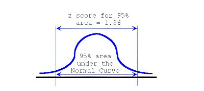
Decision rules for the normal curve approximation
If the calculated value for the z score (the Normal Curve Approximation) is within the boundaries of the critical values (-1.96) to (+1.96) {values greater than (-1.96) but less than (+1.96)} then we would say that the value falls within our region of accepting the null hypothesis and therefore state that the events were random. If the calculated value for the z score (the Normal Curve Approximation) is outside the boundaries of the critical values (-1.96) to (+1.96) {values less than (-1.96) but greater than (+1.96)} then we would say that the value falls outside our region of accepting the null hypothesis. Therefore, we must reject the null hypothesis and state that the events did not occur at random, rather, the events followed a distinct pattern.
The standardized scores (or z scores) are ratio scores based on the difference between any score within a set of scores and the measure of central tendency for that set of scores, divided by the standardized error attributed to that set of scores; as shown in the formula: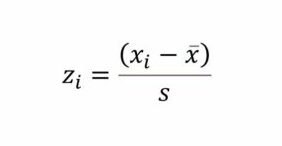
A sample data set to compute z scores
In the following sample data we can convert the raw scores from this data set to a set of z scores.
| [latex]x_i[/latex] | [latex](x_i - \overline x)[/latex] | [latex]\Delta[/latex] | [latex](x_i - \overline x)^2[/latex] | [latex]z_i =[/latex] [latex] (x_i - \overline x)\over s_i[/latex] | [latex]z_i[/latex] |
|---|---|---|---|---|---|
| 13 | 13 – 31.2 | -18.2 | 331.24 | 13-31.2/15.91 | -1.14 |
| 19 | 19 – 31.2 | -12.2 | 148.84 | 19-31.2/15.91 | -0.77 |
| 30 | 30 – 31.2 | -1.2 | 1.44 | 30-31.2/15.91 | -0.08 |
| 43 | 43 – 31.2 | 11.8 | 139.24 | 43-31.2/15.91 | 0.74 |
| 51 | 51 – 31.2 | 19.8 | 392.04 | 51-31.2/15.91 | 1.25 |
So notice in this table the conversion of the raw data to the z scores creates a new set of data that ranges from -1.14 to 1.25.
