
Measuring Correlation, Association, Reliability and Validity
35 Computing the Pearson Product Moment Correlation Coefficient
Defining the Correlation Coefficient for Continuous Data: the Pearson Product Moment Correlation Coefficient
Pearson’s Product Moment Correlation Coefficient is aptly named for the mathematical computational steps that are used to produce the outcome. First, the computation is based on the multiplication of variables, which result in generating a product. Second, the variables, labelled x and y, are computed as independent statistical moments, whereby each score is evaluated against the variable’s algebraic measure of centrality of the group scores, a.k.a. the mean. In this way, the correlation coefficient provides the researcher with an estimate of a relationship between two dependent variables.
The outcome estimate of the Pearson Product Moment Correlation Coefficient does NOT imply cause or causality between the two variables. Rather, the outcome estimate is merely an estimate of how closely two variables describe independent responses for a sample. The correlation coefficient is calculated by combining the estimates of variance on each of the separately measured variables of interest.
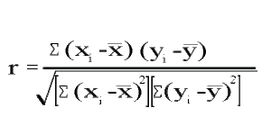
Specifically, the correlation coefficient is a ratio score that ranges from -1.00 to +1.00 and is created from a cross product:
![]()
as the numerator term and then adjusted through division by the error term in the denominator, which is the square root of the product of the sum of squares for the x variable and the sum of squares for the y variable, as shown here:![]()
The formula to compute the Pearson product-moment correlation coefficient is shown here:
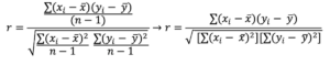
When presented graphically, the paired measures of the x and y variables for the set of scores are represented as a single point within the graphing space. The calculation of the correlation coefficient describes the mathematical relationship between the x and y variable pairs are associated within a geometric space. The following three graphs illustrate the extremes of the Pearson Product Moment Correlation Coefficients for the relationships between x and y variable pairs. In Figure 1, the relationship illustrates a Pearson Product Moment Correlation Coefficient as extreme positive with an r value of 1.00. In Figure 2, the relationship illustrates an extreme negative r value of -1.00. In Figure 3, the relationship is shown as a Pearson Product Moment Correlation Coefficient of zero, or no mathematical relationship between each participant’s paired x and y scores.
Figure 1. Representation of the Pearson Product Moment Correlation Coefficient as r=1.00
In the figure above, the cluster of paired scores on the variable x and the variable y are presented in a positive direction within the graphing space. For each individual’s score on the x variable there is an equal score on the y variable relative to the scale of scores. This means that a correspondingly high score on the y variable matches a high score on the x variable; and similarly a correspondingly low score on the y variable matches a low score on the x variable. When the x and y variables as represented as a single point in the graphing space the resulting image suggests a positive correlation between the variables x and y for the set of participants’ scores.
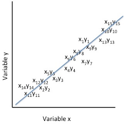
Figure 2. Representation of the Pearson Product Moment Correlation Coefficient as r= -1.00
In the figure above, the cluster of paired scores on the variable x and the variable y are presented in a negative direction within the graphing space. For each individual’s score on the x variable, there is an inverse score on the y variable relative to the scale of scores. This means that a correspondingly high score on the y variable matches a low score on the x variable, and similarly, a correspondingly low score on the y variable matches a high score on the x variable. When the x and y variables as represented as a single point in the graphing space the resulting image suggests a negative correlation between the variables x and y for the set of participants’ scores.
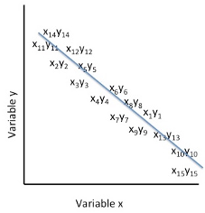
Figure 3. Representation of the Pearson Product Moment Correlation Coefficient as r= 0.00
In Figure 3, above, the cluster of paired scores on the variable x and the variable y are presented as having no definitive direction within the graphing space. For each individual’s score on the x variable, there is no corresponding score on the y variable relative to the scale of scores. In this instance, the x and y variables are simply represented as pairs of scores within the graphing space. No relationship exists when there is complete randomness in the scoring by an individual on the x and on the y variables and thereby do not depict a relationship between the two variables for the set of participants’ scores.
The correlation coefficient provides the researcher with an estimate of a relationship between two variables. The Pearson Product Moment Correlation Coefficient does NOT imply cause or causality between the two variables. Rather, the measure is merely an estimate of how closely two variables describe independent responses for a sample. The correlation coefficient is calculated by combining the measures of variance on each of the separately measured variables, as shown in the following formula:
A SAS Example
Consider the following data set, with 6 participants measured on two separate variables. Your intention is to determine if the group measures on VAR_1 are similar to the group measures of VAR_2. For those of you that need more tangible labels, let’s consider that VAR_1 represents IQ scores and that VAR_2 represents SHOE SIZE.
So that our query is simply, is there a relationship between IQ scores and SHOE SIZE. In order to analyze these data, you create the following SAS program which produces the output shown below.
SAS Code to produce Pearson Correlation Coefficient and A Line of Best Fit in a Scatterplot
DATA CORREX1;
TITLE ‘CORRELATION BETWEEN 2 MEASURES IN SAME PERSON’;
INPUT ID VAR1 VAR2;
LABEL VAR1=’MEASURE FOR VARIABLE 1′
VAR2=’MEASURE FOR VARIABLE 2′;
DATALINES;
001 55 7
002 77 9
003 88 10
004 92 10.5
005 100 11
006 105 12
;
RUN;
PROC UNIVARIATE; VAR VAR1 VAR2;
PROC CORR PEARSON; VAR VAR1 VAR2;
PROC SGPLOT NOAUTOLEGEND DATA= CORREX1;
TITLE1 “SCATTER PLOT OF CORRELATION BETWEEN VAR1 AND VAR2”;
TITLE2 “LINE OF BEST FIT ADDED TO SCATTERPLOT”;
REG Y=VAR1 X=VAR2;
RUN;
Output from PROC CORR with Corresponding Line of Best Fit in a Scatterplot
Correlation between 2 measures in the same person using the SAS PROC CORR Procedure. Table 1. Simple Statistics
| Variable | N | Mean | Std Dev | Sum | Minimum | Maximum |
| Measure for Var_1 (IQ scores) |
6 | 86.16667 | 18.10433 | 517.00000 | 55.00000 | 105.00000 |
| Measure for Var_2 Shoe Size |
6 | 9.91667 | 1.74404 | 59.50000 | 7.00000 | 12.00000 |
Table 2. Matrix of Pearson Correlation Coefficients, N = 6, Prob > |r| under H0: Rho=0
| IQ scores (Var_1) |
Shoe Size (Var_2) | |
| IQ scores (Var_1) | 1.00000
|
r= 0.99500
p <.0001 |
| Shoe Size (Var_2) | r= 0.99500
p <.0001 |
1.00000
|
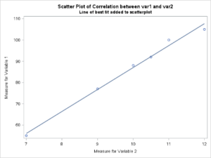
The results indicate that there is a strong correlation between IQ scores and shoe size as indicated by the correlation coefficient value in Table 2 of the SAS output in the scatterplot, above. The reported correlation coefficient (r value) was 0.995. which is considered statistically significant (p<0.0001)[1]. The r value indicates that as a group the data on each variable are traveling in the same direction. In other words, low IQ scores were associated with small shoe sizes and high IQ scores were associated with larger shoe sizes.
Another SAS Working Example
Consider the following comparison of VO2 maximum tests to illustrate the computations for the Pearson product-moment correlation coefficient.
An individual’s ability to perform maximal re-synthesis of ATP is often determined from their estimated VO2 maximum. Yet the true estimate of VO2 maximum requires an individual to undergo an extensive performance test in a “clinical or laboratory” setting.
Further, because physical fitness is often established from the VO2 maximum, researchers strive to develop approaches that can provide a suitable estimate for VO2 maximum without requiring the laboratory test. To this end, several “field tests” have been presented as reliable and valid proxies for the laboratory estimate of VO2 maximum.
The validity of field-tests for VO2 maximum as effective measures of true physiological functioning within this system are based on the linear relationship between heart rate and oxygen consumption. Since the changes in heart rate match the changes in aerobic metabolism, an individual’s ability to respire can be predicted indirectly by heart rate rather than the direct determination of oxygen utilization from a controlled laboratory setting.
Laboratory tests for VO2 maximum typically require that the individual runs or walks on a treadmill, or cycles on a standard bicycle ergometer while expired air is collected and the oxygen concentration in the expired air, is measured. The field tests, however, can use several stimulus modalities (e.g. walking, running, stepping, and cycling) and rather than measure the oxygen concentration in expired air, the technician simply records heart rate at specific stages of the exercise stress test. The relationship between field-tests and a declared “gold standard” is determined by comparing the statistical probability of the association between the predictive nature of the field test and a baseline reference standard measured in the laboratory.
In determining the accuracy of a clinical or diagnostic test, researchers compare the performance of subjects on the selected diagnostic (field) test against the “gold standard”. In the following example, this clinical epidemiological approach was used to determine the accuracy of field tests for predicting maximal oxygen consumption against a laboratory standard treadmill test (Bruce protocol). The field tests included the Cooper’s 12-minute run, the Astrand-Rhyming bicycle test, the Canadian Aerobic Fitness Test, and the one-mile walking test. A sample of the results for each test is presented in the table, below.
Table of VO2 Maximum Estimates For A Sample Of Ten Individuals On 5 Different Procedures
| Subject | treadmill VO2 max ml/kg/min |
12-minute run VO2 max ml/kg/min |
Bicycle ergometer VO2 max ml/kg/min |
Step test VO2 max ml/kg/min |
1-mile walk test VO2 max ml/kg/min |
| 01 | 47 | 33 | 44 | 57 | 45 |
| 02 | 36 | 19 | 53 | 53 | 43 |
| 03 | 55 | 25 | 49 | 61 | 47 |
| 04 | 39 | 41 | 23 | 56 | 44 |
| 05 | 57 | 27 | 50 | 58 | 45 |
| 06 | 46 | 39 | 52 | 61 | 53 |
| 07 | 43 | 36 | 55 | 57 | 44 |
| 08 | 29 | 31 | 42 | 53 | 42 |
| 09 | 54 | 28 | 44 | 56 | 44 |
| 10 | 37 | 44 | 54 | 57 | 45 |
The following computations illustrate the application of the Pearson product-moment correlation coefficient to the oxygen consumption data shown above.
STEP 1: Select two variables to compareà, for example, we will begin with VO2 measured with the treadmill test versus VO2 measured with the 1-mile walk test. The mean for the scores on the treadmill, which in this example we designate as the x variable is 44.3 (± 9.23), and the scores on the walk test, which in this example we designate as the y variable and is 45.2 (± 3.04).
![]()
The mean score for the variable x and the mean score for the variable y are used independently in Step 2: computing variance for each selected variable.
STEP 2: Compute the sum of squares for the variance elements of each selected variable, separately, as shown below:![]()
| Scores on “x” treadmill |
||
| 47 | 47 – 44.3 = 2.7 | (47 – 44.3)2= 7.29 |
| 36 | 36 – 44.3 = -8.3 | (36 – 44.3)2= 68.89 |
| 55 | 55 – 44.3 = 10.7 | (55 – 44.3)2= 114.49 |
| 39 | 39 – 44.3 = -5.3 | (39 – 44.3)2= 28.09 |
| 57 | 57 – 44.3 = 12.7 | (57 – 44.3)2= 161.29 |
| 46 | 46 – 44.3 = 1.7 | (46 – 44.3)2= 2.89 |
| 43 | 43 – 44.3 = -1.3 | (43 – 44.3)2= 1.69 |
| 29 | 29 – 44.3 = -15.3 | (29 – 44.3)2= 234.09 |
| 54 | 54 – 44.3 = 9.7 | (54 – 44.3)2= 94.09 |
| 37 | 37 – 44.3 = -7.3 | (37 – 44.3)2= 53.29 |
| = 0 | = 766.01 |
| Scores on “y” the walk test |
||
| 45 | 45 – 45.2= -0.2 | (45 – 45.2)2= 0.04 |
| 43 | 43 – 45.2 = -2.2 | (43 – 45.2)2= 4.84 |
| 47 | 47 – 45.2 = 1.8 | (47 – 45.2)2= 3.24 |
| 44 | 44 – 45.2 = -1.2 | (44 – 45.2)2= 1.44 |
| 45 | 45 – 45.2 = -0.2 | (45 – 45.2)2= 0.04 |
| 53 | 53 – 45.2 = 7.8 | (53 – 45.2)2= 60.84 |
| 44 | 44 – 45.2 = -1.2 | (44 – 45.2)2= 1.44 |
| 42 | 42 – 45.2 = -3.2 | (42 – 45.2)2= 10.24 |
| 44 | 44 – 45.2 = -1.2 | (44 – 45.2)2= 1.44 |
| 45 | 45 – 45.2 = -0.2 | (45 – 45.2)2= 0.04 |
| = 0 | = 83.6 |
STEP 3: Compute the cross products of x and y using: [latex](x_i - \overline{x})(y_i - \overline{y})[/latex]
| participant | [latex](x_i - \overline{x})(y_i - \overline{y})[/latex] |
| 01 | 2.7 * -0.2 = -0.54 |
| 02 | -8.3 * -2.2 = 18.26 |
| 03 | 10.7 * 1.8 = 19.26 |
| 04 | -5.3 * -1.2 = 6.36 |
| 05 | 12.7 * -0.2 = -2.54 |
| 06 | 1.7 * 7.8 = 13.26 |
| 07 | -1.3 * -1.2 = 1.56 |
| 08 | -15.3 * -3.2 = 48.96 |
| 09 | 9.7 * -1.2 = -11.64 |
| 10 | -7.3 * -0.2 =1.46 |
STEP 4: Compute the denominator of the correlation coefficient using the square root of the product of the sum of squares for the x and the y variables.
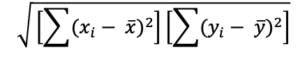
The specific values can be taken from the computations above where the ![]() = 766.01 and the
= 766.01 and the ![]() = 83.6 The denominator term is thus the square root of: SQRT(766.01 x 83.6) = SQRT(64038.44) = 253
= 83.6 The denominator term is thus the square root of: SQRT(766.01 x 83.6) = SQRT(64038.44) = 253
STEP 5: Compute the correlation coefficient by substituting the values from that which was calculated, above.

In our example, the correlation coefficient computed for the relationship between the VO2 on the treadmill and the VO2 on the 1 mile walk test = 0.37
Verifying Our Computations with SAS
The data set used in the example above included two columns of data: the VO2 max scores recorded for each participant on the treadmill test and the 1-mile walk test. The columns were separated by a tab character which we denote in our INFILE statement with the command: delimiter=’09’x . The data set has three variables: id, treadmill scores and 1-mile walk test scores.
raw data set for three variables
01 47 45
02 36 43
03 55 47
04 39 44
05 57 45
06 46 53
07 43 44
08 29 42
09 54 44
10 37 45
The SAS program written for SAS Studio to compute the correlation coefficient for the relationship between the scores on the treadmill and the 1-mile walk test is shown here:
SAS Code to produce Pearson Correlation Coefficient for treadmill and the 1-mile walk test
DATA CORR1(LABEL= ‘CORRELATION COEFFICIENTS’);
TITLE ‘PRACTICE DATA SET TO COMPUTE CORRELATION COEFFICIENTS’;
INFILE ‘/FOLDERS/DATASETS/CORR1.DAT’ DELIMITER=’09’X ;
* THE DATA IN THE FILE CORR1.DAT ARE TAB DELIMITED;
INPUT ID 1-3 @4 TRDMILL ONEMLWLK;
PROC CORR; VAR TRDMILL ONEMLWLK;
RUN;
Output from the SAS PROC CORR PROCEDURE
| Variable | N | Mean | Std Dev | Sum | Minimum | Maximum |
| trdmill | 10 | 44.30000 | 9.22617 | 443.00000 | 29.00000 | 57.00000 |
| Onemlwlk | 10 | 45.20000 | 3.04777 | 452.00000 | 42.00000 | 53.00000 |
| trdmill | Onemlwlk | |
| Trdmill | r= 1.00000 | r = 0.37301
p < 0.2884 |
| Onemlwlk | r = 0.37301
p < 0.2884 |
r = 1.00000 |
Testing the significance of the sample correlation coefficient
When we compute the r statistic (correlation coefficient) the relationship that we observe is specific to the sample from which the data were drawn. If we wish to compute the population parameter of a correlation coefficient, that is the extension of the statistic for the sample to the parameter in the population, then our next step is to compute the rho statistic – rho is the population parameter estimate of the correlation coefficient and it is determined using a t test with (n-2 degrees of freedom).
To determine if the computed correlation coefficient is equal to 0 as in the null hypothesis test: H0: r = 0 at p<0.05 we use the following equation:
[latex]t = r \sqrt\frac{n-2}{1-r^2}[/latex]
with the degrees of freedom (npairs – 2).
Therefore, in the example presented above, the correlation coefficient was r=0.37, and the sample size was n=10. The t value to evaluate the population parameter is shown below with degrees of freedom = (npairs – 2) = (10 – 2) = 8.

The t critical value for t=1.126 with df=8 is 2.31 for p<0.05. Therefore, because our t statistic is less than the critical value, we would accept the null hypothesis at p<0.05 and suggest that in this sample, the estimate of the relationship between treadmill VO2 maximum scores with 1-mile walk test scores is not an estimate of the true population parameter (i.e. the rho score). Finally, in addition to computing the significance of the correlation coefficient, we can also determine the strength of the correlation coefficient. Typically, the decision rule concerning the strength of a correlation coefficient is as follows: if the absolute value of r is low (<0.7) then we say that is no correlation, but if the absolute value is (>0.7) then we say that there is a correlation between the scores on the variable x and the scores on the variable y.
Strength of the Correlation
The strength of the correlation is determined by squaring the value of r (the correlation coefficient) and multiplying the result by 100. Taken in this way, we are able to express the bivariate correlation (i.e. the relationship between two variables) as a percent of variance that is explained between the two variables.
For example, if we square the correlation coefficient computed for the relationship between the VO2 on the treadmill and the VO2 on the 1-mile walk test, as follows:
r = 0.37 and r2 = 0.139 x 100 = approximately 14%
We can then say that the variable x and the variable y have a very low relationship and when this relationship is expressed in terms of variance, then the variables x and y in this example share only about 14% of the variance between these two variables, leaving more than 86% of the variance between these two variables unexplained.
Conversely, if we had computed a correlation coefficient of 0.9 between the variable x and the variable y then we would say that there is a strong relationship and could express the variance shared by these two variables as follows:
r = 0.9 and r2 = 0.81 x 100 = approximately 81% explained variance.
Here is what we covered in this chapter
In this chapter you were introduced to:
- The Pearson Product Moment Correlation Coefficient which we defined as an estimate of a relationship between two dependent variables.
- We also stated, explicitly, that the outcome estimate of the Pearson Product Moment Correlation Coefficient does NOT imply cause or causality between the two variables.
- The correlation coefficient, which is represented by the letter ‘r’ expresses a positive relationship between two variables (a bivariate relationship) when the r-value is greater than 0 and less than 1, a negative relationship between two variables when the r value is less than 0 and greater than -1, and no relationship when the r-value is in close proximity to 0 and is deemed to be not significant based on the formula: [latex]t = r \sqrt\frac{n-2}{1-r^2}[/latex] with degrees of freedom (n_pairs – 2).
- In the examples presented here we observed how SAS code enables us to not only produce the estimates of the relationship but also produce a visual representation of the data from the two variables being compared and include a representative line of best fit.
Practice Question for This Chapter
So, you’ve decided to take on a positive lifestyle that, among other behaviours, includes changes in diet and exercise. You are really interested in eating smarter and becoming more active to enhance your cardiovascular efficiency. You want to become physically fit. But, how does one know that they are achieving a higher level of physical fitness? For some individuals, they may perceive that they are achieving a state of physical fitness by simply looking in the mirror after bathing and observing a change in body shape. While this approach invokes a response, it is not a good indicator of the intrinsic cardiovascular changes that you may actually be gaining. An alternative to mirror gazing is to measure heart rate response after performing a physically demanding task. For example, for many individuals measuring heart rate after climbing stairs is a good indication that their involvement in physical fitness pursuits is having a positive change in cardiovascular dynamics. While this approach seems extremely simple it is certainly easily measured, and changes are easily recognized.
In the Canadian Physical Activity Test novice fire fighters are evaluated on a stepping test in which they are required to walk on a stepping ergometer (a treadmill like device that simulates stepping) at a stepping rate of 60 steps per minute for three minutes while wearing two 5.67 kg weights on their shoulders. The weights are used to represent wearing fully charged air packs during an actual fire-fighting event. In the following fictitious experiment, data were collected from a sample of 20 individuals ranging in ages from 40 to 60 years that climbed 180 steps at a rate of 60 steps per minute. Heart rates were measured in each participant within the first minute following activity and 3 minutes following the activity. The number of minutes of physical activity in which the individual was engaged per week was also recorded for each participant.
In this exercise compute the correlation coefficient of the relationship between the reported number of minutes of physical activity in which the individual reportedly averaged per week with both the immediate heart rate response to stair climbing (1-minute post-exercise heart rate) and the 3-minute recovery heart rate following the stair climbing exercise. Produce the correlation coefficient in table form and a graphical representation of each bivariate relationship. Likewise, determine the significance of the relationship using the formulae shown above.
Table of Raw Data from the Mock Stair Climbing Experiment
| Participant | Age | Amount of exercise per week (minutes) | 1-minute post-exercise heart rate (bpm) | 3-minute post-exercise heart rate (bpm) |
| 01 | 56 | 420 | 144 | 75 |
| 02 | 56 | 315 | 163 | 84 |
| 03 | 45 | 210 | 178 | 97 |
| 04 | 49 | 210 | 147 | 66 |
| 05 | 47 | 140 | 144 | 88 |
| 06 | 56 | 105 | 142 | 101 |
| 07 | 53 | 70 | 180 | 117 |
| 08 | 59 | 350 | 144 | 53 |
| 09 | 44 | 90 | 190 | 106 |
| 10 | 47 | 315 | 144 | 57 |
| 11 | 46 | 420 | 124 | 55 |
| 12 | 56 | 315 | 133 | 54 |
| 13 | 55 | 210 | 158 | 77 |
| 14 | 59 | 210 | 147 | 86 |
| 15 | 60 | 140 | 164 | 98 |
| 16 | 40 | 105 | 162 | 101 |
| 17 | 53 | 70 | 176 | 117 |
| 18 | 54 | 350 | 144 | 59 |
| 19 | 40 | 90 | 184 | 126 |
| 20 | 60 | 315 | 134 | 77 |
Some hints to get you started
DATA hrCorr01;
TITLE ‘CORRELATION BETWEEN REPORTED WEEKLY PHYSICAL ACTIVITY AND HR RESPONSES TO STAIR CLIMBING’;
INFILE ‘/HOME/USERNAME/YOURFOLDERS/HRCORR.DAT’ DELIMITER= ’09’X ;
/* NOTES – IF YOU USE THE INFILE STATEMENT AS SHOWN ABOVE THEN BE SURE TO
CHANGE THE USERNAME AND FOLDERS WHERE THE DATA RESIDE, ALSO SINCE THIS EXAMPLE IS TAKEN DIRECTLY FROM THE TABLE BE SURE TO SET DELIMITER TO TAB BETWEEN VALUES */
INPUT ID AGE EX_MIN HR_1MIN HR_3MIN;
PROC CORR PEARSON; VAR EX_MIN HR_1MIN HR_3MIN; RUN;
PROC SGPLOT NOAUTOLEGEND DATA= hrCorr01;
TITLE1 “SCATTERPLOT OF CORR BETWEEN REPORTED WEEKLY PHYSICAL ACTIVITY AND IMMEDIATE POST EXERCISE HEART RATE RESPONSE TO STAIR CLIMBING”;
TITLE2 “LINE OF BEST FIT ADDED TO SCATTERPLOT”;
LABEL EX_MIN =’REPORTED EXERCISE IN MINUTES PER WEEK’
HR_1MIN =’IMMEDIATE POST EXERCISE HEART RATE’;
REG Y= EX_MIN X= HR_1MIN; RUN;
PROC SGPLOT NOAUTOLEGEND DATA= hrCorr01;
TITLE1 “SCATTERPLOT OF CORR BETWEEN REPORTED WEEKLY PHYSICAL ACTIVITY AND 3 MINUTE POST EXERCISE HEART RATE RECOVDERY TO STAIR CLIMBING”;
TITLE2 “LINE OF BEST FIT ADDED TO SCATTERPLOT”;
LABEL EX_MIN =’REPORTED EXERCISE IN MINUTES PER WEEK’
HR_3MIN =’3 MINUTE RECOVERY HEART RATE’;
REG Y= EX_MIN X= HR_3MIN;
* Explain the outcome of your calculation in terms related to the original research question.
- Note: just because the p value extends beyond 0.01 you need only to report p<0.01 ↵
