
| SES GRPS | Frequency | Percent | Cumulative Frequency |
Cumulative Percent |
|---|---|---|---|---|
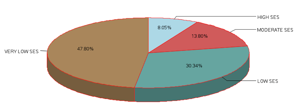
| HIGH SES | 165 | 8.05 | 165 | 8.05 |
| MODERATE SES | 283 | 13.80 | 448 | 21.85 |
| LOW SES | 622 | 30.34 | 1070 | 52.20 |
| VERY LOW SES | 980 | 47.80 | 2050 | 100.00 |
Goodness of Fit and Related Chi-Square Tests
15 Introducing the Goodness of Fit Chi-Square
So you are asking yourself, “goodness of fitting what to what?”
The chi-square (pronounced “kie” square) is an extremely useful, non-parametric statistical technique, that allows a researcher to compare responses from a sample to expected responses in a – hypothetical distribution of responses for a population. Hence the name goodness of fit test.
The chi-square goodness of fit test can be used to evaluate data at all variable levels, but because the currency of this test is count data, the goodness of fit test can be used to compute nominal and ordinal data.
The chi-square test evaluates data in the form of counts or frequencies, as in the number of responses within a given category, or the number of people who responded a given way to a specific question, or the number of cases across outcome categories.
The goodness of fit chi-square for one sample with four categories
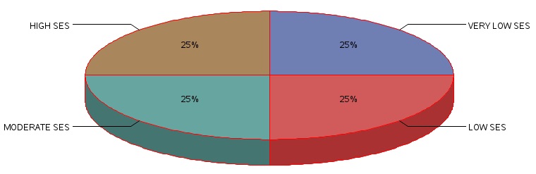
In the following example, we consider the goodness of fit chi-square with four response categories. In this problem, we are studying a cohort of cancer patients to determine if cancer was more likely to be diagnosed in patients who are in a low-income category, based on socio-economic status (SES) quartiles. We begin by establishing that the expected distribution of cancer patients within the community is equally distributed across the four income categories so that in any community 25% of our population are in the highest SES category, 25% are in the moderate SES category, 25% are in the low SES income category, and 25% are in the very low SES category.
Proportional Distribution of Sample Across Socioeconomic Categories
However, in the observed data set for our sample of cancer patients, we recorded the following distribution of patients.
|
Highest SES 25% |
Moderate SES 25% |
Lower SES 25% |
Very Low SES 25% |
|
Data from the community sample of cancer patients collected over a 10 year period in a community with an average population of greater than 1 million households |
|||
|
165 patients |
283 patients |
622 patients |
980 patients |
The null hypothesis for this study is stated in an unbiased way so that each SES quartile is expected to have an equal percentage of households with cancer patients. Therein, the term f(k) = refers to the frequency or number of patients within the quartile indicated by the subscript (k). Since we have four groups representing four quartiles then (k) ranges from 1 to 4.
H0: f1 = f2 = f3 = f4
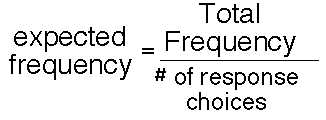
Since we have a total sample size of N = 2050, then each cell of the SES quartiles is expected to have a frequency (an expected number of patients) equal to 512.5 individuals.
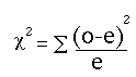
The chi-square formula to test the null hypothesis is:

The equation measures how closely an observed set of responses (the“o” for “observed”) matches an expected set of responses (the “e” for “expected”).
So then how do we calculate the items that we use in the chi-square equation?
The observed frequencies are simply taken from the data recording sheet, but the expected frequencies
are computed from the following formula:
Another way to view the computation of the expected frequencies is to consider the null hypothesis which stated that:
H0: f1= f2= f3= f4
and multiply the total frequency by the probability associated with each category, as in the following computations.
2050 x 0.25 = 512.5
The chi-square is then used to compute whether or not the observed distribution fits a hypothetical or expected distribution. This can be accomplished by setting up the following table below:
|
|
|
|
= 788.24 |
|
Response Category |
Observed Frequency |
Expected Frequency |
(Obs – Exp)2 ÷ Exp |
|
1: High SES |
165 |
512.5 |
235.62 |
|
2: Moderate SES |
283 |
512.5 |
102.77 |
|
3: Low SES |
622 |
512.5 |
23.40 |
|
4: Very Low SES |
980 |
512.5 |
425.45 |
In this calculation for a one-sample scenario with 4 outcome categories, we see that the Here the chi-square statistic is: 788.24. So what does this mean?
To evaluate the meaning of the variable we calculated for the Chi-square we need to review the decision rule for the Chi-square statistic, and shown here.
|
Chi-Square decision rule (one-sample chi-square test): The computed score is referred to as the chi-square observed. After computing the chi-square observed value, determine the chi-square critical score from a table of chi-square values. The chi-square critical score represents what we should expect to observe for a distribution with five responses. The critical value is determined by computing the degrees of freedom for our response set. The computation of the degrees of freedom is: degrees of freedom = k possible responses -1 degrees of freedom = 5-1 degrees of freedom = 4 and the chi-square critical value for degrees of freedom of 4 at p<0.05 = 9.49 If the chi-square observed value is GREATER THAN the chi-square critical value of 9.49, we must reject the null hypothesis and state that the distribution of responses across the four categories IS NOT EQUAL. A large chi-square value, that is a value that exceeds the chi-square critical value demonstrates that the outcome is less likely to occur by chance. |
The chi-square statistic is computed as 788.24.
We, therefore, compare the chi-square observed value of 788.24 against a chi-square expected, based on the expected probability level and the degrees of freedom. In the k=4 chi-square, the degrees of freedom are: degrees of freedom = “k” possible responses -1, so that given k=4, then the degrees of freedom is 4-1 = 3 and at p<0.05 the chi-square critical value is 7.82. Therefore, since our chi-square observed value of 788.24 exceeds the chi-square critical (7.82) we reject the null hypothesis and state that the distribution of cancer patients is not equally distributed across the SES categories, and given the numbers we observed we can state that in this sample, the number of cancer patients in the very low SES group was significantly greater than the number of cancer patients in the high socio-economic category.
The following is the SAS code used to analyze the data in the scenario above.
PROC FORMAT;

VALUE SLICE 1='HIGH SES' 2='MODERATE SES' 3='LOW SES' 4='VERY LOW  SES';

DATA GFIT_1;
INPUT SESGRP N_PATNTS;
/* DEFINE THE AXIS CHARACTERISTICS */
AXIS1 LABEL=("SES CATEGORIES")
VALUE=(JUSTIFY=CENTER);
AXIS2 LABEL=(ANGLE=90 "ACTUAL NUMBER OF PATIENTS")
ORDER=(0 TO 1000 BY 100)
MINOR=(N=3);
AXIS3 LABEL=(ANGLE=90 "SES CATEGORIES");

AXIS4 LABEL=("ACTUAL NUMBER OF PATIENTS") ;
DATALINES;
1 165
2 283
3 622
4 980
;
/* HERE WE USE THE OPTION SUMVAR TO GRAPH THE SUM OF THE FREQ */
PROC FREQ ORDER=DATA; TABLES SESGRP/CHISQ CL CELLCHI2;
WEIGHT N_PATNTS;
FORMAT SESGRP SLICE. ;
TITLE 'FREQUENCY DISTRIBUTION FOR PROPORTION OF PATIENTS IN EACH SES GROUP';
TITLE2 'ONE SAMPLE GOODNESS OF FIT EXAMPLE FOR K=4';
RUN;
The output for Chi-square computation is shown here:
The FREQUENCY procedure including the chi-square statistic to evaluate the null hypothesis H0: f1 = f2 = f3 = f4.
| Chi-Square Test for Equal Proportions |
|
|---|---|
| Chi-Square | 788.2400 |
| DF | 3 |
| Pr > ChiSq | <.0001 |
The SAS code to produce the pie chart is as follows:
PROC FORMAT;VALUE SLICE 1='HIGH SES' 2='MODERATE SES' 3='LOW SES' 4='VERY LOW SES';PROC GCHART DATA=GFIT_1;PIE3D SESGRP/SUMVAR=N_PATNTS TYPE=SUM DISCRETE PERCENT=insideCOUTLINE=RED WOUTLINE=1 FILL=SOLID SLICE =ARROW CLOCKWISENOLEGEND NOHEADING VALUE=NONE;FORMAT SESGRP SLICE. ;TITLE1 'PIE CHART FOR PROPORTION OF PATIENTS IN EACH SES GROUP';PATTERN1 COLOR = LIGHTBLUE;RUN;PIE CHART FOR PROPORTION OF PATIENTS IN EACH SES GROUP
Webulator Form 1:
The following is a Goodness of Fit Webulator for k= 4 responses In the table above we used the values for socioeconomic status:
| HIGH SES | 165 |
|---|---|
| MODERATE SES | 283 |
| LOW SES | 622 |
| VERY LOW SES | 980 |
Enter these data into the webulator below for each of your four options and then click the button labelled compute expected frequencies. This will produce the sum of the four values that you entered and compute the expected frequency for the values in the table.
The important value from this Webulator is the computed chi-square score. The computed score is referred to as the chi-square observed. After computing the chi-square observed value, determine the chi-square critical score from a table of chi-square values. The chi-square critical score represents what we should expect to observe for the distribution with “k” responses. The critical value is determined by computing the “degrees of freedom” for our response set.
The computation of the degrees of freedom is: degrees of freedom = “k” possible responses -1
degrees of freedom = 4-1 –> degrees of freedom = 3
and the “chi-square critical value” for degrees of freedom of “3” at p<0.05 = 7.815
If the “chi-square observed value ” is › the “chi-square critical value of 7.815”, we must reject the null hypothesis and state that the distribution of responses across the response categories IS NOT EQUAL.
