Often referred to as distribution-free statistics, non-parametric statistics are used when the data may not demonstrate the characteristics of normality (i.e. follow a normal distribution). Non-parametric statistics are used with nominal data, where the response set can be converted to counts of events, and the measurement scale is ignored.

Non-parametric statistics can be used when data are converted to ranks.

Non-parametric statistics are most useful when data are not normally distributed, or when sample sizes are so small that the representativeness of the sample to the population is questionable.

The standard scores (a.k.a. z scores)

In statistics, when we want to standardize scores within a distribution, we simply transform the scores using a common denominator to create a ratio level measurement. One of the simplest methods for standardizing scores is to produce an estimate referred to as the “z” score.

The z score is referred to as the standard normal value or standard normal deviate because it follows the standard normal distribution and represents the standardized estimate of difference of any score within a random variable from the mean of the random variable. The standard normal distribution is represented by the normal curve. The standard normal distribution has a mean = 0 and a standard deviation = 1.

Given that this exercise was to demonstrate to the research community how the set of sample scores are associated with the true set of population scores, then we need to find some way of relating the sample distribution to the population distribution (or how is the set of scores for the sample related to the set of scores for the population). One way to illustrate such a relationship is to standardize the scores for both the sample distribution and the population distribution. In statistics when we want to standardize an estimate we typically relate the estimate to a measurement standard called the normal curve.

The normal curve is a graphical representation of the standard normal distribution (ie. the frequency distribution graph of an expected distribution of scores within a “normal population”). By using the normal curve, researchers can describe how closely their sample distribution represents a population distribution.

Understanding the role of the normal curve is important to inferential statistics. The normal curve is a graphical presentation of the frequency distribution for a set of standardized (or adjusted) scores. For any set of z scores, a percentile estimate can be attributed to each z score. This has been shown several times and is commonly known as the Z table of estimates or the table for the normal curve. Conversely then for any percentile, we could determine a standardized estimate or a z score. That is, we could determine the z score for a percent of confidence such as the 95% confidence value.

The normal curve approximation

We call the computation of the z score, the normal curve approximation since we are trying to estimate where our events fall within the set of possible outcomes represented by the normal curve. The set of hypothetical expected outcomes for the normal curve is presented in the figure below. Notice the critical region in which we accept the null hypothesis is within the boundaries (-1.96) to (+1.96). The region to accept the null hypothesis generally accounts for 95% of the expected outcomes, allowing 5% of the outcomes to be outside the region of acceptance (shown here as 2.5% in each of the tails).

Illustration of the area under the normal curve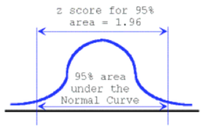

Decision rules for the normal curve approximation

If the calculated value for the z score (the Normal Curve Approximation) is within the boundaries of the critical values (-1.96) to (+1.96) {values greater than (-1.96) but less than (+1.96)} then we would say that the value falls within our region of accepting the null hypothesis and therefore state that the events were random. If the calculated value for the z score (the Normal Curve Approximation) is outside the boundaries of the critical values (-1.96) to (+1.96) {values less than (-1.96) but greater than (+1.96)} then we would say that the value falls outside our region of accepting the null hypothesis. Therefore, we must reject the null hypothesis and state that the events did not occur at random, rather, the events followed a distinct pattern.