
SAS Programming
12 Graphing Data for Effective Presentations
Learner Outcomes
After reading this chapter you should be able to:
- Organize data from various sources, and especially identify the specific variables that comprise a data set and separate data into independent and dependent measures.
- Present your data in a graphical format to convey your message to the reader by identifying the level of measurement for each of the variables within the data set and organize the data appropriately for the type of graph or table selected
- Select from a variety of graphing and charting features in SAS to create an appropriate visual presentation of variables in your dataset and thereby demonstrate when a graph of a particular type is most appropriate
- Prepare your data set for graphing and charting by transposing from wide to narrow or narrow to wide
- Create a simple SAS program to produce different types of graphs and tables
- Add specific features such as axis labels, legends, and colors to enhance your graphical presentation of variables in the data set
Preamble
Producing graphical images is one of the most important features of conveying the statistical message. Face it, statistics is a hard area to wrap your brain around because it is based on the complexity of mathematically derived outcomes. What is the chance of picking the correct lottery number? How many people do I need in my study to know that I can represent the population? What is the best outcome from the randomized clinical trial that I should achieve before I decide that the vaccine is effective? Chance, probability, estimation, hypotheses, confidence, prediction, these are all complex concepts in which we only estimate the likelihood of our accuracy.
Statistics is the science that helps us to create knowledge based on the information attributed to the facts that make up our datasets.
Graphing is an approach that enables us to bring the data from the abstractness of a fact to the reality of a contextualized image. With a graph, we view the image and then interpret the meaning of the image from our understanding of the mathematical system that the image represents.
In applying statistics, and more specifically learning statistics, graphs are essential.
Creating a Visual Presentation of Your Data
In this section, we will organize data from various sources, and especially identify the specific variables that comprise a data set and separate data into independent and dependent measures. The examples here will enable us to present data in a graphical format to convey our message to the reader by identifying the level of measurement for each of the variables within the data set and organize the data appropriately for the type of graph or table selected.
Graphing is a useful technique to illustrate:
- the shape of data sets relative to how scores are distributed
- relationships or associations between variables within or between data sets
- the magnitude of differences for numbers within and between datasets
In this section, we will use several different examples of graphing and charting features in SAS to create the appropriate visual presentation of variables in our dataset and thereby demonstrate when a graph of a particular type is most appropriate. In addition, we will work through examples that prepare data sets for graphing and charting by transposing from wide to narrow or narrow to wide, as well as adding specific features such as axis labels, legends, and colors to enhance your graphical presentation of variables in the data set.
Creating a Vertical Bar Chart to Represent John Snow’s Natural Experiment
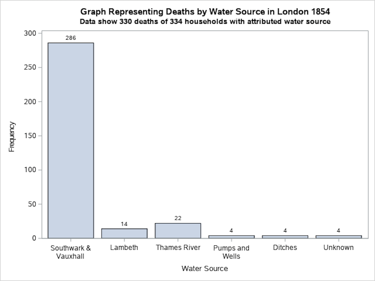
In this first example, we will use the PROC SGPLOT command to create a vertical bar graph to represent the data that John Snow reported for the water source by household in his 1854 surveillance during the London Cholera epidemic. The data are discrete frequencies of households which are then plotted against the source of drinking water for the household. The SAS code used to generate this vertical bar chart is presented below the image.
In this SAS graphing program we create a vertical bar graph to represent the data that John Snow reported for the water source by household in his 1854 surveillance during the London Cholera epidemic. The data are discrete frequencies of households and these are plotted against the source of drinking water for the household.
The SAS Code to generate the Vertical Bar Chart above.
options pagesize=55 linesize=120 center date;
PROC FORMAT;
VALUE SLICE 1 = ‘Southwark & Vauxhall’
2 = ‘Lambeth’
3 = ‘Thames River’
4 = ‘Pumps and Wells’
5 = ‘Ditches’
6 = ‘Unknown’;
data snow1;
input source deaths ;
label Source = ‘Water Source’;
datalines;
1 286
2 14
3 22
4 04
5 04
6 04
;
run;
proc sgplot data=snow1; vbar source / freq=deaths datalabel;
FORMAT source SLICE. ;
run;
 |
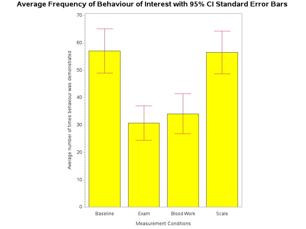
In the following program we added error bars based on 95% confidence interval calculations to each vertical bar. The SAS code is annotated with comments throughout.
SAS Program to Create Vertical Bar Chart with error bars
proc format;
value cndfmt 1 = ‘Baseline’ 2 = ‘Exam’ 3 = ‘Blood Work’ 4 = ‘Scale’;
data behave;
input Code Cond bhvscr @@;
xvar=cond; yvar=bhvscr;
label xvar=’Measurement Conditions’;
label yvar=’Average number of times behaviour was demonstrated’;
datalines;
01 1 79 01 2 54 01 3 51 01 4 85 02 1 21 02 2 15 02 3 23 02 4 80
03 1 37 03 2 14 03 3 18 03 4 38 04 1 61 04 2 21 04 3 13 04 4 79
05 1 32 05 2 30 05 3 34 05 4 58 06 1 60 06 2 30 06 3 15 06 4 50
07 1 78 07 2 53 07 3 67 07 4 53 08 1 67 08 2 42 08 3 47 08 4 48 09 1 41
09 2 10 09 3 28 09 4 28 10 1 72 10 2 52 10 3 33 10 4 24 11 1 62
11 2 21 11 3 60 11 4 47 12 1 44 12 2 46 12 3 54 12 4 52 13 1 32
13 2 11 13 3 25 13 4 32 14 1 39 14 2 37 14 3 12 14 4 36 15 1 55 15 2 20
15 3 23 15 4 49 16 1 62 16 2 22 16 3 28 16 4 49 17 1 83 17 2 34
17 3 22 17 4 43 18 1 86 18 2 14 18 3 47 18 4 80 19 1 54 19 2 47 19 3 77
19 4 44 20 1 76 20 2 57 20 3 24 20 4 88 21 1 56 21 2 14 21 3 18 21 4 59
22 1 37 22 2 43 22 3 39 22 4 75 30 1 28 30 2 13 30 3 15 30 4 81 31 1 94
31 2 31 31 3 69 31 4 90 52 1 90 51 2 55 52 3 26 52 4 70 53 1 48 53 2 14
53 3 29 53 4 53 54 1 47 54 2 29 54 3 24 54 4 34
;
/* Define the axis characteristics */
axis1 offset=(0,70) minor=none; axis2 label=(angle=90);
pattern1 color = yellow;
/* The term pattern1 refers to the first item to be graphed. If there were two variables being graphed then we we use pattern1 and pattern3. */
proc sort; by xvar;
proc gchart data = behave;
vbar xvar/ type=MEAN errorbar=BOTH clm=95
sumvar=yvar discrete raxis=axis2 cerror=crimson cr=biv;
format xvar cndfmt.;
/* Define the title */
title1 ‘Average Frequency of Behaviour of Interest with 95% CI Standard Error Bars ‘;
run;
More Simple Barcharts — Graphing data as a Frequency Distribution Bar Chart
In the following examples, we use SAS commands to create a three-dimensional vertical bar chart and a horizontal bar chart with a frequency table of the data. In this SAS code, we include formatting commands for the graphical output – defining the characteristics of each axis – prior to having the SAS program read the data set.
Using GCHART to Produce A Vertical Bar Chart
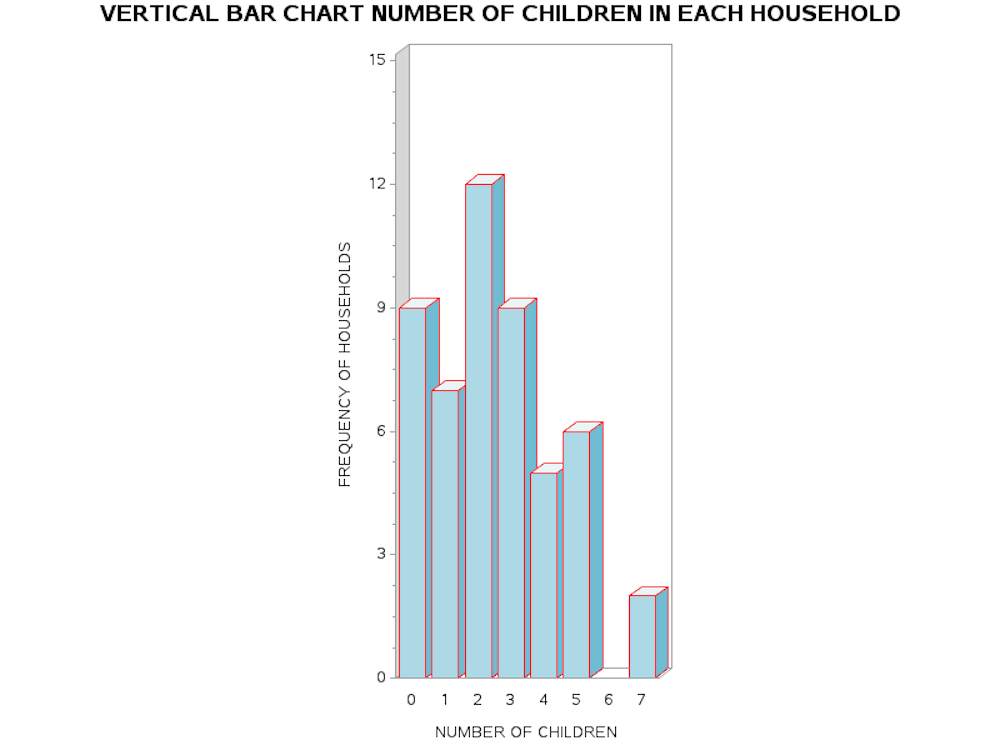 |
| DATA FAMILIES; INPUT NKIDS HSEHLD; /* DEFINE THE AXIS CHARACTERISTICS */ AXIS1 LABEL=("NUMBER OF CHILDREN") VALUE=(JUSTIFY=CENTER); AXIS2 LABEL=(ANGLE=90 "FREQUENCY OF HOUSEHOLDS") ORDER=(0 TO 15 BY 3) MINOR=(N=3); AXIS3 LABEL=(ANGLE=90 "NUMBER OF CHILDREN"); AXIS4 LABEL=("FREQUENCY OF HOUSEHOLDS") ; DATALINES; PROC GCHART DATA=FREQ4_3; |
The essential SAS processing command to produce the vertical bar chart is PROC GCHART. However, the important commands to discriminate the independent and dependent variables are given in the command line: VBAR3D NKIDS/SUMVAR=HSEHLD TYPE=SUM DISCRETE. Here we tell SAS to read the variable NKIDS as the categorical independent variable, while HSEHLD is the dependent variable and is read by the option SUMVAR= HSEHLD. We include the second option TYPE=SUM to indicate that the values entered are actually the sum scores for each category of the independent variable.
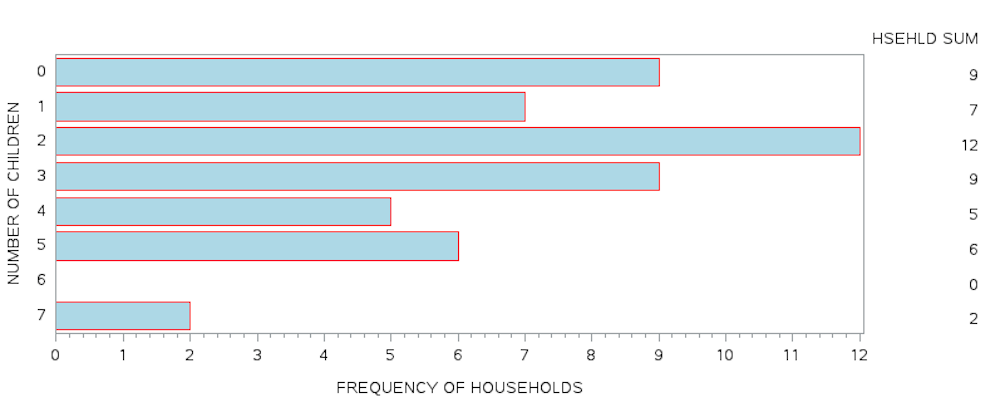
Using the same data from the SAS program above and adding two new AXIS labels we can generate a horizontal bar chart with the frequency values included at the end of each horizontal bar. Notice in both the vertical and horizontal bar charts, the length of the bar is proportional to the value of the frequency.
Horizontal Bar Chart with Frequency Values Included
 |
| DATA FAMILIES; INPUT NKIDS HSEHLD @@; /* DEFINE THE AXIS CHARACTERISTICS */ AXIS3 LABEL=(ANGLE=90 "NUMBER OF CHILDREN"); DATALINES; |
Notice in the input statement, the variables are defined and two @ symbols are used to hold the cursor at the line until all values are entered in sequence.
INPUT NKIDS HSEHLD @@;
This style for data entry economizes space in programming.
In the following example, we return to the HDX dataset to observe the total number of cases of the Ebola virus across selected countries. These data are based on the actual reports of cases and deaths related to the 2014 West Africa Ebola Outbreak.
Sample Data Of Total Cases Of Ebola Virus Across Selected Countries
| Country | Case definition | Total cases | Total deaths | Country report date |
|---|---|---|---|---|
| Guinea | Confirmed | 2384 | 1422 | 2014-12-27 |
| Probable | 275 | 275 | ||
| Suspected | 36 | 0 | ||
| All | 2695 | 1697 | ||
| Liberia | Confirmed | 3108 | .. | 2014-12-24 |
| Probable | 1773 | .. | ||
| Suspected | 3096 | .. | ||
| All | 7977 | 3413 | ||
| Sierra Leone | Confirmed | 7326 | 2366 | 2014-12-27 |
| Probable | 287 | 208 | ||
| Suspected | 1796 | 158 | ||
| All | 9409 | 2732 |
The SAS program and corresponding output from the analysis is presented below. Notice that only the data for confirmed, probable and suspected cases are being used in the dataset. These data represent the summary of counts whereby the units of measurement are the total number of cases and the total number of deaths.
SAS Program to Create a Frequency Distribution for Ebola Outbreak
DATA GRAPH1;
INPUT COUNTRY $ 1-12 DEF $ 15-23 CASES 26-29;
LABEL DEF=’DEFINITION OF CASES’;
DATALINES;
GUINEA CONFIRMED 2384
GUINEA PROBABLE 275
GUINEA SUSPECTED 36
LIBERIA CONFIRMED 3108
LIBERIA PROBABLE 1773
LIBERIA SUSPECTED 3096
SIERRA LEONE CONFIRMED 7326
SIERRA LEONE PROBABLE 287
SIERRA LEONE SUSPECTED 1796
;
PROC SORT; BY COUNTRY;
PROC FREQ; TABLES COUNTRY/OUT=CASEPCT; WEIGHT CASES;
RUN;
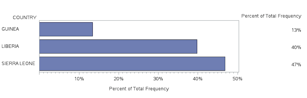
The output from the PROC FREQ procedure is shown here.
| COUNTRY | Frequency | Percent | Cumulative Frequency |
Cumulative Percent |
| GUINEA | 2695 | 13.42 | 2695 | 13.42 |
| LIBERIA | 7977 | 39.72 | 10672 | 53.14 |
| SIERRA LEONE | 9409 | 46.86 | 20081 | 100.00 |
In the code above we produce an output file that represents the percent value of the cases based on the sum of cases in each country. For example, all of the cases for GUINEA regardless of whether the cases were PROBABLE, SUSPECTED, or CONFIRMED, equal 2695 which represents 13.42 percent of the total number of cases. The total number of cases across all countries is reported in the last row of the Cumulative Frequency column and is 20081.
Below, the output data file (DATA=CASEPCT) is used in a PROC GCHART procedure to produce a horizontal bar chart using the SUMVAR option with the data from the PERCENT column.
| PROC FORMAT; PICTURE PCTFMT (ROUND) 0-HIGH=’000%’;
PROC GCHART DATA=CASEPCT; HBAR COUNTRY/ SUMVAR = PERCENT; FORMAT PERCENT PCTFMT.; RUN; |
Creating a Line Graph to Summarize Data
In this program, we will use the SAS PROC GPLOT functions to observe “at a glance” a comparison of the unadjusted differences in life expectancy at birth for males versus females in Canada, based on data reported since 1994. The data used in this example range from an initial value of 74.9 years for males and 80.9 years for females in 1994, to life expectancy scores of 79.8 years for males and 83.9 years for females, in 2015. Here we see that at each year of reporting life expectancy estimates, the females are predicted to live longer than males, on average.
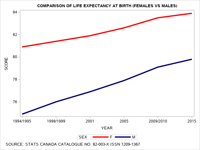
SAS SGPLOT to Produce Comparison of Life Expectancy Scores
PROC FORMAT;
VALUE $SXFMT ‘F’=’FEMALE’ ‘M’=’MALE’;
VALUE YRFMT 1=’1994/1995′ 2=’1998/1999′ 3=’2001′ 4=’2005′ 5=’2009/2010′ 6=’2015′;
VALUE SRCFMT 1=’UNADJUSTED LIFE EXPECTANCY’ 2=’HEALTH ADJUSTED LIFE EXPECTANCY’;
LABEL SCORE= ‘LIFE EXPECTANCY AT BIRTH’;
LABEL YEAR= ‘YEAR OF REPORTING’;
DATA CH7FIG1;
INPUT ID SEX $ YEAR SOURCE SCORE @@;
DATALINES;
01 M 1 1 74.9 02 M 2 1 76.0 03 M 3 1 76.9 04 M 4 1 77.9 05 M 5 1 79.1 M 06 6 1 79.8 07 M 1 2 65.0 08 M 2 2 67.4 09 M 3 2 67.3 10 M 4 2 68.1
11 M 5 2 69.3 12 M 6 2 69.0 13 F 1 1 80.9 14 F 2 1 81.4 15 F 3 1 81.9
16 F 4 1 82.6 17 F 5 1 83.5 18 F 6 1 83.9 19 F 1 2 67.8 20 F 2 2 70.1
21 F 3 2 69.8 22 F 4 2 70.6 23 F 5 2 71.3 24 F 6 2 70.5
;
TITLE2 ‘COMPARISON OF LIFE EXPECTANCY AT BIRTH (FEMALES VS MALES)’;
FOOTNOTE1 J=L ” SOURCE: STATS CANADA CATALOGUE NO. 82-003-X ISSN 1209-1367″;
AXIS1 ORDER=(1990 TO 2015 BY 5) OFFSET=(2,2) LABEL=NONE
MAJOR=(HEIGHT=2) MINOR=(HEIGHT=1) ;
AXIS2 ORDER=(50 TO 100 BY 5) OFFSET=(0,0) LABEL=NONE
MAJOR=(HEIGHT=2) MINOR=(HEIGHT=1);
LEGEND1 LABEL=NONE POSITION=(TOP CENTER INSIDE)
MODE=SHARE;
RUN;
PROC SORT; BY SEX;
PROC SGPLOT;
SERIES X = YEAR Y = SCORE/GROUP=SEX lineattrs=(thickness=4);
XAXIS TYPE = DISCRETE;
styleattrs datacontrastcolors=(RED NAVY)
datalinepatterns=(SOLID);
WHERE SOURCE=1 ;
FORMAT YEAR YRFMT. SOURCE SRCFMT. ;
RUN;
Adding the WHERE command to restrict output
In the following line graph, we observe the Health Adjusted Life Expectancy, also referred to as HALE data comparison between males and females changes the contours of the lines for the predicted values of the female and male response data. Again these data range from first reports in 1994 taken from the National Population Health Survey and the Canadian Census in 1993 to 1995 to data from the Canadian Community Health Survey, as well as the NPHS and Census up to and including 2015 (Bushnik, Tjepkema, Martel, 2018)[1].
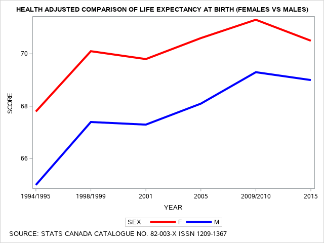
The SAS program to produce the line graph above includes the PROC SGPLOT statement and the command WHERE SOURCE=1; This restricts the processing of the graphing procedure to only select the unadjusted life expectancy values from the dependent variable SCORE. When we change the command WHERE SOURCE=2; then we change the output to only consider health adjusted values from the dependent variable SCORE.
Here we use the PROC FORMAT feature to ensure that the data are converted to explanatory labels and these labels are included in the graphs.
SAS SGPLOT to produce Health Adjusted Comparison of Life Expectancy Scores
This program is incorporating the WHERE command to restrict output to a subgroup.
PROC SORT; BY SEX;
PROC SGPLOT; SERIES X = YEAR Y = SCORE/GROUP=SEX
lineattrs=(thickness=4);XAXIS TYPE = DISCRETE;
styleattrs datacontrastcolors=(RED BLUE)
datalinepatterns=(SOLID);
WHERE SOURCE=2 ;
FORMAT YEAR YRFMT. SOURCE SRCFMT. ;
RUN;
[1]Bushnik, T., Tjepkema, M., & Martel, L., Health-adjusted life Expectancy in Canada, Statistics Canada. Catalogue no. 82-003-X ISSN 1209-1367
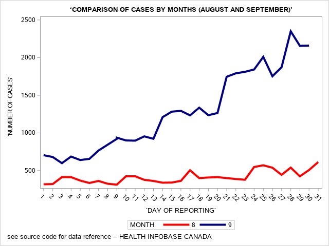
Let’s add one more line graph here to show the comparison of the number of reported cases for COVID-19 for the months of August and September in Canada. Note, the PROC SORT command is extremely important here.
The SAS program and corresponding output are shown below.
PROC FORMAT;
VALUE $MNFMT 08=’August’ 09=’September’;
DATA A3Q1C;
INPUT MONTH DAY CASES @@;
TITLE2 ‘NUMBER OF CORONAVIRUS CASES IN THE MONTHS OF AUGUST AND SEPTEMBER 2020’;
LABEL CASES= ‘NUMBER OF CASES’;
LABEL DAY= ‘DAY OF REPORTING’;
DATALINES;
08 01 319 08 08 326 08 15 342 08 22 389 08 29 425
08 02 322 08 09 314 08 16 364 08 23 379 08 30 508
08 03 414 08 10 425 08 17 505 08 24 548 08 31 614
08 04 414 08 11 425 08 18 401 08 25 571
08 05 368 08 12 378 08 19 409 08 26 539
08 06 336 08 13 363 08 20 414 08 27 444
08 07 363 08 14 340 08 21 401 08 28 540
09 01 705 09 09 922 09 15 1283 09 22 1792 09 29 2157
09 02 681 09 09 938 09 16 1294 09 23 1812 09 30 2160
09 03 599 09 10 901 09 17 1234 09 24 1843
09 04 687 09 11 898 09 18 1336 09 25 2010
09 05 641 09 12 955 09 19 1236 09 26 1753
09 06 656 09 13 923 09 20 1265 09 27 1873
09 07 767 09 14 1210 09 21 1746 09 28 2350
;
TITLE2 ‘COMPARISON OF CASES BY MONTHS (AUGUST AND SEPTEMBER)’;
FOOTNOTE1 J=L “see source code for data reference — HEALTH INFOBASE CANADA”;
/*
* https://health-infobase.canada.ca/covid-19/epidemiological-summary-covid-19-cases.html
*/
AXIS1 ORDER=(1 TO 31 BY 1) OFFSET=(22) LABEL=NONE MAJOR=(HEIGHT=2) MINOR=(HEIGHT=1) ;
AXIS2 ORDER=(100 TO 2500 BY 100) OFFSET=(00) LABEL=NONE MAJOR=(HEIGHT=2) MINOR=(HEIGHT=1);
LEGEND1 LABEL=NONE POSITION=(TOP CENTER INSIDE) MODE=SHARE;
RUN;
PROC SORT; BY DAY;
PROC SGPLOT;
SERIES X = DAY Y = CASES / GROUP=MONTH lineattrs=(thickness=4);
FORMAT MONTH MNFMT. ;
XAXIS TYPE = DISCRETE;
styleattrs datacontrastcolors=(RED NAVY)
datalinepatterns=(SOLID);
RUN;
Plotting Coronq Virus cases: Data for Canada Months of August and September
Creating a Pie Chart to Represent Summary Data
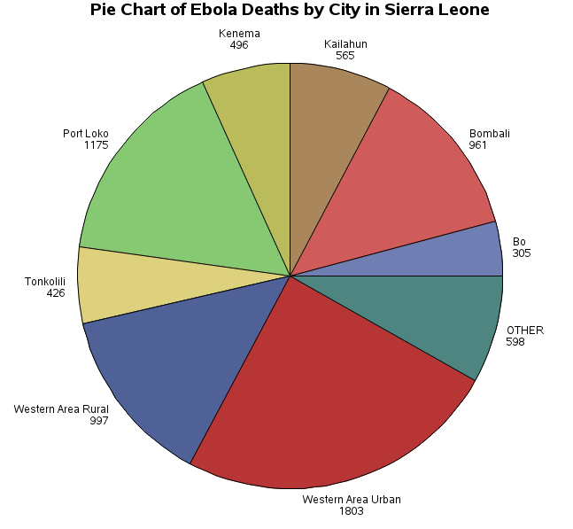
In the following example, we present a pie chart of the data from The Humanitarian Data Exchange (url: https://data.hdx.rwlabs.org/) a project from the United Nations Office for the Coordination of Humanitarian Aid (url: http://www.unocha.org/).
On January 15th, 2016 the World Health Organization declared the country of Sierra Leone as Ebola-free. However, by that time Sierra Leone had recorded approximately 4000 deaths from the Ebola Virus. In this second example, we will generate a pie chart. The data are based on confirmed cases of Ebola for Sierra Leone by region from 2014 to December 28, 2014. The data represent the cumulative deaths since the recognized beginning of the Ebola virus outbreak in April 2014.
 |
|---|
| /* ****************************************************************** * SAS CODE TO PRODUCE PIE CHART FOR EBOLA RELATED * DEATHS IN CITIES OF SIERRA LEONE * BE SURE TO CHECK COLUMN ALIGNMENT ******************************************************************* */. OPTIONS PAGESIZE=55 LINESIZE=120 CENTER DATE; |
| WESTERN AREA URBAN 1803 400 WESTERN AREA RURAL 997 112 KAMBIA 108 22 PORT LOKO 1175. 219 TONKOLILI 426 41 KONO 176 70 KAILAHUN 565 3 KENEMA 496 2 PUJEHUN 31 0 KOINADUGU 97 11 BO 305 36 BONTHE 5 1 BOMBALI 961 81 MOYAMBA 181 11 |
| ; RUN; TITLE1 'PIE CHART OF EBOLA DEATHS BY CITY IN SIERRA LEONE'; |
The data for this example are taken from the HDX: The Humanitarian Data Exchange to represent deaths from the Ebola outbreak in Sierra Leone in 2014.
Producing Bubble Plots
SOURCE: HDX: The Humanitarian Data Exchange [1]
In the following example data set the cumulative number of health-care workers deaths by Ebola Disease Virus are reported. These data were extracted from WHO: Ebola Response Roadmap Situation Reports, the data are based on extraction from data reported on 24 December 2014. Here we can plot the total deaths from these data by country, and within each country by month and use appropriate axes titles and legend. The data are presented first in the table below and then as two separate bubble plots. The size of the bubbles represents the frequency value for the total number of deaths reported.
Number Of Health-Care Workers Deaths By Ebola Disease Virus (Sept 2014 - Dec 2014)
| Country | Total deaths | Month | Country | Total deaths | Month | Country | Total deaths | Month |
|---|---|---|---|---|---|---|---|---|
| Guinea | 27 | Sept | Sierra Leone | 81 | Sept | Liberia | 103 | Oct |
| Liberia | 81 | Sept | Guinea | 35 | Sept | Nigeria | 5 | Oct |
| Sierra Leone | 31 | Sept | Liberia | 95 | Sept | Sierra Leone | 95 | Oct |
| Guinea | 30 | Sept | Nigeria | 5 | Sept | Guinea | 43 | Oct |
| Liberia | 85 | Sept | Sierra Leone | 81 | Sept | Liberia | 123 | Oct |
| Nigeria | 5 | Sept | Guinea | 40 | Oct | Nigeria | 5 | Oct |
| Sierra Leone | 31 | Sept | Liberia | 96 | Oct | Sierra Leone | 101 | Oct |
| Guinea | 35 | Sept | Nigeria | 5 | Oct | Guinea | 46 | Nov |
| Liberia | 87 | Sept | Sierra Leone | 95 | Oct | Liberia | 157 | Nov |
| Nigeria | 5 | Sept | Guinea | 41 | Oct | Nigeria | 5 | Nov |
| Guinea | 56 | Nov | Mali | 2 | Nov | Sierra Leone | 102 | Nov |
| Liberia | 172 | Nov | Guinea | 59 | Nov | Guinea | 55 | Nov |
| Sierra Leone | 105 | Nov | Liberia | 174 | Nov | Liberia | 170 | Nov |
| Nigeria | 5 | Nov | Sierra Leone | 106 | Nov | Nigeria | 5 | Nov |
| Guinea | 51 | Nov | Nigeria | 5 | Nov | Sierra Leone | 104 | Nov |
| Liberia | 162 | Nov | Guinea | 62 | Dec | Guinea | 62 | Dec |
| Nigeria | 5 | Nov | Liberia | 174 | Dec | Liberia | 174 | Dec |
| Sierra Leone | 102 | Nov | Sierra Leone | 106 | Dec | Sierra Leone | 106 | Dec |
| Nigeria | 5 | Dec | Liberia | 177 | Dec | Nigeria | 5 | Dec |
| Mali | 2 | Dec | Sierra Leone | 110 | Dec | Mali | 2 | Dec |
| Guinea | 72 | Dec | Nigeria | 5 | Dec | Guinea | 72 | Dec |
| Liberia | 177 | Dec | Mali | 2 | Dec | Liberia | 177 | Dec |
| Sierra Leone | 109 | Dec | Sierra Leone | 110 | Dec | Sierra Leone | 109 | Dec |
| Nigeria | 5 | Dec | Nigeria | 5 | Dec | Nigeria | 5 | Dec |
| Mali | 2 | Dec | Liberia | 177 | Dec | Mali | 2 | Dec |
| Guinea | 72 | Dec | Mali | 2 | Dec | Guinea | 72 | Dec |
Data Source: (url: https://data.hdx.rwlabs.org/) a project from the United Nations Office for the Coordination of Humanitarian Aid (url: http://www.unocha.org/)
The SAS program to analyze these data is presented below. Notice that the dataset presented above used three columns: Country, Total Deaths, and Months, which are repeated three times, using the following input statement. The double trailing @@ symbols hold the pointer at the end of the line to ensure that the data read as three variables repeated three times.
Sample Code:
INPUT COUNTRY $ TOTDTH MONTH $ @@;
In this way, the SAS program reads the data and produces the output for the entire dataset. Notice that we precede the input statement by declaring the length of the contents of the variable COUNTRY to be more than 12 characters in length.
SAS code to Produce Bubble Chart
DATA GRAPH2;
LENGTH COUNTRY $12.;
INPUT COUNTRY $ TOTDTH MONTH $ @@;
LABEL TOTDTH =’NUMBER OF DEATHS’;DATALINES;
<DATA GOES HERE>
Sample of the raw data:
Sierra_Leone 31 Sept Liberia 95 Sept Sierra_Leone 95 Oct
…
RUN;
PROC SORT; BY COUNTRY;
PROC FREQ DATA=GRAPH2;WEIGHT TOTDTH; TABLES MONTH*COUNTRY;
RUN;
* NOTICE THE WEIGHT STATEMENT IS USED WHEN THE RAW DATA ARE SUMS;
PROC SGPLOT DATA=GRAPH2;
TITLE1 ‘BUBBLE PLOT’;
TITLE2 ‘EXAMPLE 1: TOTAL DEATHS BY COUNTRY’;
BUBBLE X = COUNTRY Y = TOTDTH SIZE = TOTDTH / GROUP = MONTH TRANSPARENCY = 0.5;
FOOTNOTE1 J=L “SOURCE: HTTPS://DATA.HUMDATA.ORG/DATASET/NUMBER-OF-HEALTH-CARE-WORKERS-DEATHS-BY-EDV”;PROC SGPLOT DATA=GRAPH2;
TITLE1 ‘BUBBLE PLOT’;
TITLE2 ‘EXAMPLE 2: TOTAL DEATHS BY MONTH’;
BUBBLE X = MONTH Y = TOTDTH SIZE = TOTDTH / GROUP = COUNTRY TRANSPARENCY = 0.5; YAXIS GRID ;
RUN;
The summary frequency distribution is presented here first.
| Month | Guinea | Liberia | Mali | Nigeria | Sierra_Leone | Total |
| Sept | f= 127
% total = 2.41 row % = 17.79 col % = 13.66 |
f= 1056
% total =20.02 row % = 48.89 col % = 41.23 |
f= 12
% total =0.23 row % = 0.56 col % = 85.71 |
f= 30
% total =0.57 row % = 1.39 col % = 35.29 |
f= 650
% total =12.32 row % = 30.09 col % = 38.60 |
f= 2160
% total =40.96 |
| Oct | f= 124
% total = 2.35 row % = 16.49 col % = 13.33 |
f= 322
% total = 6.11 row % = 42.82 col % = 12.57 |
f= 0
% total = 0.00 row % = 0.00 col % = 0.00 |
f= 15
% total = 0.28 row % = 1.99 col % = 17.65 |
f= 291
% total = 5.52 row % = 38.70 col % = 17.28 |
f= 752
row % = 14.26
|
| Nov | f= 267
% total = 5.06 row % = 16.20 col % = 28.71 |
f= 835
% total = 15.83 row % = 50.67 col % = 32.60 |
f= 2
% total = 0.04 row % = 0.12 col % = 14.29 |
f= 25
% total = 0.47 row % = 1.52 col % = 29.41 |
f= 519
% total = 9.84 row % = 31.49 col % = 30.82 |
f= 1648
row % =31.25
|
| Dec | f= 412
% total = 7.81 row % = 19.07 col % = 44.30 |
f= 1056
% total = 20.02 row % = 48.89 col % = 41.23 |
f= 12
% total = 0.23 row % = 0.56 col % = 85.71 |
f= 30
% total = 0.57 row % = 1.39 col % = 35.29 |
f= 650
% total = 12.32 row % = 30.09 col % = 38.60 |
f= 2160
row % = 40.96
|
| Total | f= 930
col % = 17.63 |
f= 2561
col % = 48.56 |
f= 14
col % = 0.27 |
f= 85
col % = 1.61 |
f= 1684
col % = 31.93 |
f= 5274
100.00 |
Bubble plots can be used to illustrate the distribution of outcomes within specific groups. In the following two graphs the data from the summary frequency table of month by country above, which showed deaths within the countries monitored across months are presented using two different grouping strategies. In the first example (bubble plot example 1) the data showing the number of deaths (Y-axis) are separated using countries as the main X-Axis variable and months as the grouping variable.
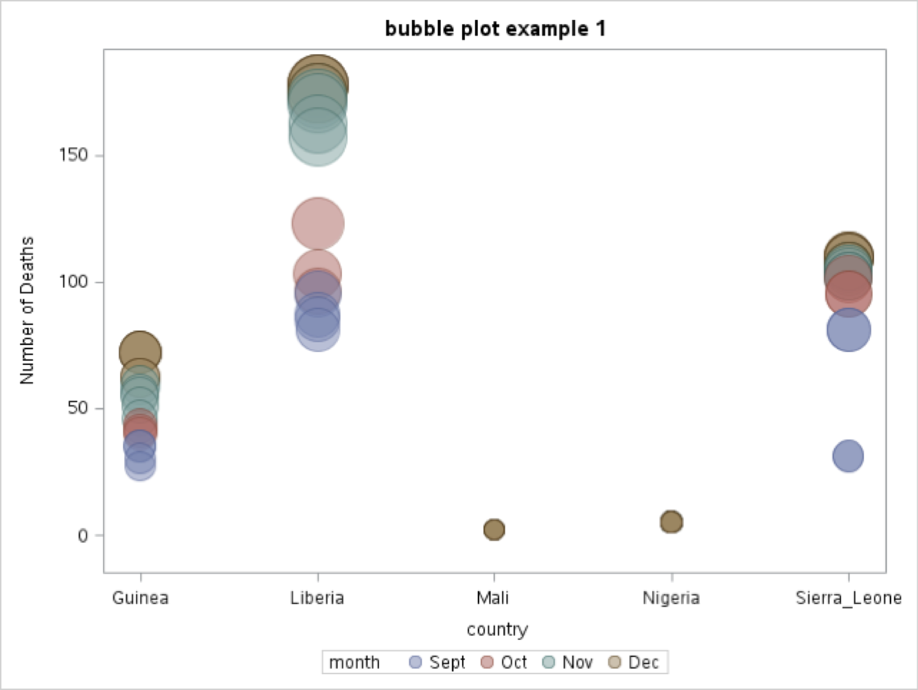 The specific SAS code is:
TITLE1 ‘BUBBLE PLOT’;
TITLE2 ‘EXAMPLE 1: TOTAL DEATHS BY COUNTRY’;
BUBBLE X = COUNTRY Y = TOTDTH SIZE = TOTDTH / GROUP = MONTH TRANSPARENCY = 0.5;FOOTNOTE1 J=L “SOURCE: HTTPS://DATA.HUMDATA.ORG/DATASET/NUMBER-OF-HEALTH-CARE-WORKERS-DEATHS-BY-EDV”;
In the second example (bubble plot example 2) the data showing the number of deaths (Y-axis) are separated using months as the main X-axis variable and country in which the deaths occurred is the grouping variable.
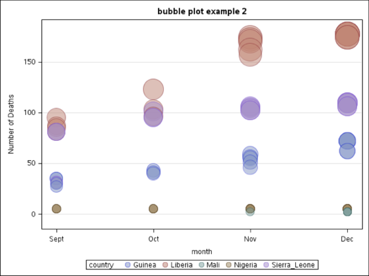
The specific SAS code is presented here. Notice we did not need to repeat the footnote statement from Bubble Plot 1 for it to be included in Bubble Plot 2 because the RUN; statement was held until the end of the program.
TITLE1 ‘BUBBLE PLOT’;
TITLE2 ‘EXAMPLE 2: TOTAL DEATHS BY MONTH’;
BUBBLE X = MONTH Y = TOTDTH SIZE = TOTDTH / GROUP = COUNTRY TRANSPARENCY = 0.5; YAXIS GRID ;
RUN;
Producing Star Charts
In this SAS graphing procedure we show how out of balance sedentary behaviour can be in comparison to other activities of daily living.
Primary healthcare has continued to support the notion that sedentary behaviours are major risk factors for most chronic diseases. In particular, there has been a growing awareness of the relationship between sitting for prolonged periods during the day as a risk factor for chronic diseases such as CVD/CHD, type II diabetes, and hypertension. The data reported here is the estimated time in non-standing related activities. We can use a star chart to demonstrate an effective approach to representing unbalanced data for a given outcome. These data are from the American Heart Foundation (2015).
The SAS code to generate a horizontal bar chart with a corresponding frequency distribution table and two different star graphs are shown below. Notice in this SAS code we predefine the length of the input data for the variable BEHAVIOR and we use a fixed input format to enter the data values for the variables TIME in columns 22 to 24 and the variable GROUP in columns 27 to 28.
DATA STARS;
LENGTH BEHAV $20.;
INPUT BEHAV $ 1-20 TIME 22-24 GRP 27-28 ;
LABEL TIME=’TIME (HOURS)’; LABEL BEHAV=’BEHAVIOUR’;
DATALINES;
MORNING_WALK 0.5 1
DRIVE_TO_WORK 1.0 1
AM_COMPUTER_TIME 4.0 1
LUNCHTIME 0.5 1
PM_COMPUTER_TIME 4.0 1
DRIVE_HOME 1.0 2
STRENGTH_TRAINING 0.5 2
DINNERTIME 0.5 2
RELAX_TV_OR_READ 4.0 2
BEDTIME 8.0 2
;
PROC GCHART;
HBAR BEHAV/SUMVAR=TIME;
TITLE1 “HOURS SPENT IN SEDENTARY BEHAVIOUR-HORIZONTAL BAR CHART”;
RUN;
PROC GCHART ;
TITLE1 “EXAMPLE STAR GRAPH 1”;
TITLE2 “HOURS SPENT IN SEDENTARY BEHAVIOUR”;
STAR BEHAV / DISCRETE SUMVAR=TIME FILL=S;
RUN;
PROC GCHART ;
STAR BEHAV / DISCRETE SUMVAR=TIME NOCONNECT;
TITLE1 “EXAMPLE STAR GRAPH 2”;
TITLE2 “HOURS SPENT IN SEDENTARY BEHAVIOUR”;
RUN;
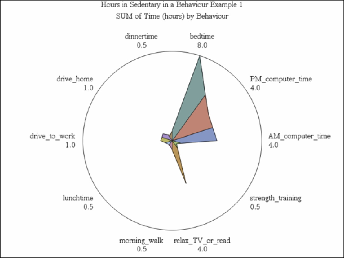
In the image above we include the FILL=S; option in the SAS code
TITLE1 “EXAMPLE STAR GRAPH 1”;
TITLE2 “HOURS SPENT IN SEDENTARY BEHAVIOUR”;
STAR BEHAV / DISCRETE SUMVAR=TIME FILL=S;
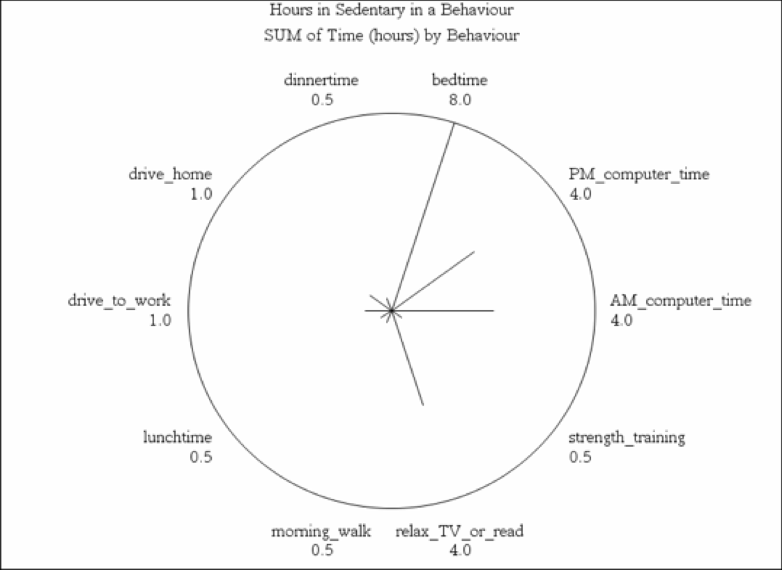
In the image above we we remove the FILL=S option and include the NOCONNECT option in the SAS code
STAR BEHAV / DISCRETE SUMVAR=TIME NOCONNECT;
TITLE1 “EXAMPLE STAR GRAPH 2”;
TITLE2 “HOURS SPENT IN SEDENTARY BEHAVIOUR”;
Preparing data for graphing by transposing datasets
In this next section, we will rotate the perspective of the data set — a term we refer to as TRANSPOSING. With the PROC TRANSPOSE feature, we can re-orient the data set from written in a wide format to a narrow format.
The wide-format of the dataset is shown in the table below. With the SAS code below we can transpose four variables into one variable. The following table is the original four variables from the raw data.
| Obs | ID | var1 | var2 | var3 | var4 |
| 1 | 7 | 0.350 | 0.326 | 0.333 | 0.333 |
| 2 | 9 | 0.346 | 0.328 | 0.318 | 0.325 |
| 3 | 10 | 0.350 | 0.352 | 0.345 | 0.355 |
| 4 | 11 | 0.345 | 0.330 | 0.341 | 0.321 |
| 5 | 13 | 0.348 | 0.342 | 0.335 | 0.330 |
| 6 | 14 | 0.347 | 0.334 | 0.342 | 0.350 |
| 7 | 15 | 0.349 | 0.325 | 0.324 | 0.327 |
| 8 | 16 | 0.338 | 0.322 | 0.334 | 0.324 |
| 9 | 18 | 0.331 | 0.329 | 0.314 | 0.335 |
| 10 | 19 | 0.342 | 0.332 | 0.323 | 0.328 |
| 11 | 20 | 0.338 | 0.318 | 0.325 | 0.331 |
SAS Code to transpose the data from a wide to a narrow format
DATA TRNSPS_W2N;
/* TRANSPOSING WIDE DATA TO NARROW DATA */
INPUT ID VAR1 VAR2 VAR3 VAR4;
DATALINES;
7 0.35 0.326 0.333 0.333
9 0.346 0.328 0.318 0.325
10 0.35 0.352 0.345 0.355
11 0.345 0.33 0.341 0.321
13 0.348 0.342 0.335 0.33
14 0.347 0.334 0.342 0.35
15 0.349 0.325 0.324 0.327
16 0.338 0.322 0.334 0.324
18 0.331 0.329 0.314 0.335
19 0.342 0.332 0.323 0.328
20 0.338 0.318 0.325 0.331
;
TITLE1 ‘TRANSPOSING FOUR VARIABLES INTO ONE VARIABLE’;
PROC SORT DATA=TRNSPS_W2N; BY ID;
TITLE2 ‘PRINT OF THE ORIGINAL FOUR VARIABLES FROM THE RAW DATA’;
PROC PRINT; VAR ID VAR1 VAR2 VAR3 VAR4 ;
RUN;
PROC TRANSPOSE DATA=TRNSPS_W2N OUT=NARROW;
BY ID;
TITLE2 ‘PRINT OF THE TRANSPOSED DATA TO A SINGLE VARIABLE’;
RUN;
PROC PRINT DATA=NARROW; VAR ID _NAME_ COL1;
RUN;
A portion of the narrow format of the data is shown here in this printout of the transposed data. Here we show the four variables as one categorical variable and one outcome variable, which can then be graphed.
| Obs | ID | _NAME_ | COL1 |
| 1 | 7 | var1 | 0.350 |
| 2 | 7 | var2 | 0.326 |
| 3 | 7 | var3 | 0.333 |
| 4 | 7 | var4 | 0.333 |
| 5 | 9 | var1 | 0.346 |
| 6 | 9 | var2 | 0.328 |
| 7 | 9 | var3 | 0.318 |
| 8 | 9 | var4 | 0.325 |
| 9 | 10 | var1 | 0.350 |
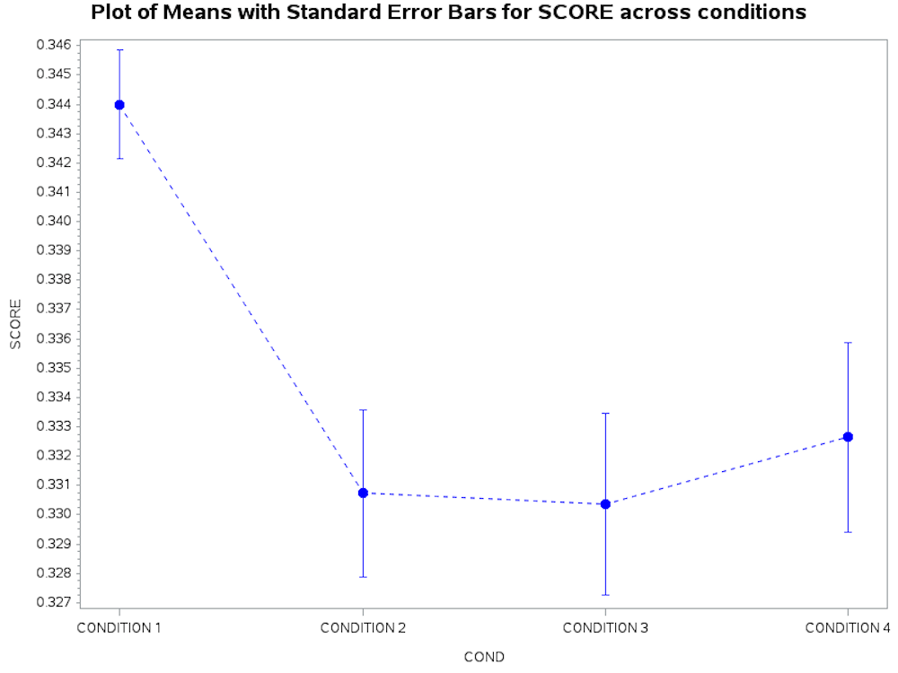
The data in the transposed table above can be used in a graph to show the response of each participant for the single dependent variable, which we called SCORE, across four measures. The SGPLOT procedure was modified from SAS SUPPORT CODE: Sample 50217: Plot means with standard error bars from calculated data for groups with PROC GPLOT[1].
SAS Code for Wide to Narrow
PROC FORMAT;
VALUE CNDFMT 1 = ‘CONDITION 1’
2 = ‘CONDITION 2’
3 = ‘CONDITION 3’
4 = ‘CONDITION 4’ ;
/* PLOT OF DEPENDENT VARIABLE AFTER TRANSPOSE TO NARROW DATA */
DATA W2N;
INPUT OBS ID COND SCORE;
/* USE THE TRANSPOSED DATASET IN A LINE GRAPH ACROSS 4 CONDITIONS */
DATALINES;
1 7 1 0.350
2 7 2 0.326
<MORE DATA HERE >
41 20 1 0.338
42 20 2 0.318
43 20 3 0.325
44 20 4 0.331
;
TITLE1 ‘TRANSPOSING FOUR VARIABLES INTO ONE VARIABLE’;
TITLE2 ‘TRANSPOSED VARIABLE AS A SINGLE RESPONSE ACROSS FOUR TIME POINTS’;
AXIS1 ORDER=(1 TO 4 BY 0.55) OFFSET=(2,2)
LABEL=NONE MAJOR=(HEIGHT=2) MINOR=(HEIGHT=1);
AXIS2 ORDER=(0.3 TO 0.4 BY 0.01) OFFSET=(0,0)
LABEL=NONE MAJOR=(HEIGHT=2) MINOR=(HEIGHT=1);
RUN;
PROC SORT DATA=W2N; BY COND;
PROC MEANS DATA=W2N NOPRINT;
BY COND;
VAR SCORE;
OUTPUT OUT=MEANSOUT MEAN=MEAN STDERR=STDERR;
TITLE1 ‘DESCRIPTIVE STATISTICS FOR SCORE ACROSS 4 CONDITIONS’;
RUN;
/* RESHAPE THE DATA TO PRESENT ONE Y VALUE FOR */
/* EACH X FOR USE WITH THE HILOC INTERPOLATION. */
DATA RESHAPE(KEEP=COND SCORE MEAN);
SET MEANSOUT;
SCORE=MEAN;
OUTPUT;
SCORE=MEAN – STDERR;
OUTPUT;
SCORE=MEAN + STDERR;
OUTPUT;
RUN;
/* DEFINE THE TITLE */
TITLE1 ‘PLOT OF MEANS WITH STANDARD ERROR BARS FOR SCORE ACROSS CONDITIONS’;
/* DEFINE THE AXIS CHARACTERISTICS */
AXIS1 OFFSET=(5,5) MINOR=NONE;
AXIS2 LABEL=(ANGLE=90);
/* DEFINE THE SYMBOL CHARACTERISTICS */
SYMBOL1 INTERPOL=HILOCTJ COLOR=BLUE LINE=2;
SYMBOL2 INTERPOL=NONE COLOR=BLUE VALUE=DOT HEIGHT=1.5;
/* PLOT THE ERROR BARS USING THE HILOCTJ INTERPOLATION */
/* AND OVERLAY SYMBOLS AT THE MEANS. */
PROC GPLOT DATA=RESHAPE;
PLOT SCORE*COND MEAN*COND / OVERLAY HAXIS=AXIS1 VAXIS=AXIS2;
FORMAT COND CNDFMT.;
RUN;
This SAS code from the transposed dataset produced the following graph.
 Transposing data from narrow to a wide format
Consider now if our data were in a long format, as in a single column with 3 categories but we wanted to reshape the data so that each of the categories became a separate measure of interest. In the following data set consisting of a categorical variable that we called employment status and a dependent variable based on household savings in the bank on January 1. Here, we will transpose the data from a long format to a wide format and convert the initial measure of interest to three variables.
The initial SAS code with data is as follows[2]:
SAS Code for Narrow to Wide
PROC FORMAT;
VALUE EMP 1= ‘FULL-TIME’ 2 = ‘PART-TIME’ 3= ‘CASUAL’;
DATA EMPSTAT;
LABEL ID = ‘PARTICIPANT ID’
EMPSTAT = ‘EMPLOYMENT STATUS’
SAVINGS = ‘SAVINGS IN BANK’;
INPUT ID 1-2 EMPSTAT 4 SAVINGS 6-9;
DATALINES;
01 3 0020
02 1 0120
03 2 0050
04 3 0030
05 3 0000
06 1 4500
07 1 8900
08 2 0540
09 3 0900
10 1 3220
11 2 0240
12 2 0400
;
PROC SORT data=EMPSTAT; BY EMPSTAT;
PROC FREQ; TABLES EMPSTAT;
FORMAT EMPSTAT EMP. ;
PROC FREQ; TABLES EMPSTAT*SAVINGS;
FORMAT EMPSTAT EMP. ;
TITLE1 ‘ FREQUENCY DISTRIBUTION FOR EMPLOYMENT STATUS’;
RUN;
PROC SORT data=EMPSTAT; BY ID;
PROC TRANSPOSE data=EMPSTAT out=NEW_WIDE prefix=GROUP_;
by ID ;
id EMPSTAT;
var SAVINGS;
RUN;
proc print data = NEW_WIDE; VAR ID GROUP_1 GROUP_2 GROUP_3;
TITLE ‘OUTPUT FOR WIDE FORMATTED DATA’;
RUN;
PROC MEANS MEAN MEDIAN STD STDERR CV; VAR GROUP_1 GROUP_2 GROUP_3;
TITLE ‘USING PROC MEANS- DESCRIPTIVE STATISTICS FOR WIDE FORMATTED DATA’;
RUN;
PROC TABULATE data = NEW_WIDE;
LABEL GROUP_1 = ‘EMPLOYED FULL TIME’
GROUP_2 = ‘EMPLOYED PART TIME’
GROUP_3 = ‘EMPLOYED CASUALLY’;
VAR GROUP_1 GROUP_2 GROUP_3;
TABLE (GROUP_1 GROUP_2 GROUP_3)* (N MEAN STD CV);
TITLE ‘USING PROC TABULATE – DESCRIPTIVE STATISTICS FOR WIDE FORMATTED DATA’;
RUN;
The SAS code above produced the following output after transposing the data from the dependent variable to produce three measures of interest which we called GROUP_1 GROUP_2 and GROUP_3. Each variable now represents the data within the specific employment category and the PROC TABULATE and PROC MEANS commands were used to produce descriptive statistics for each separate dependent measure.
FREQUENCY DISTRIBUTION FOR EMPLOYMENT STATUS
| EMPLOYMENT STATUS | FREQUENCY | PERCENT | CUMULATIVE FREQUENCY | CUMULATIVE PERCENT |
| FULL TIME | 4 | 33,33 | 4 | 33.33 |
| PART-TIME | 4 | 33.33 | 8 | 33.33 |
| CASUAL | 4 | 33.33 | 12 | 100 |
USING PROC MEANS TO PRODUCE DESCRIPTIVE STATISTICS FOR WIDE FORMATTED DATA
The MEANS Procedure
| Variable | Mean | Median | Std Dev | Std Error | Coeff of Variation |
| GROUP_1
GROUP_2 GROUP_3 |
4185.00
307.50 237.50 |
3860.00
320.00 25.00 |
3641.70
210.93 441.84 |
1820.85
105.47 220.92 |
87.01
68.60 186.04 |
USING PROC TABULATE –DESCRIPTIVE STATISTICS FOR WIDE FORMATTED DATA
DESCRIPTIVE STATISTICS CALCULATED WITH PROC TABULATE
| EMPLOYED FULL TIME | |||
| N | MEAN | STANDARD DEVIATION | COEFFICIENT OF VARIATION |
| 4 | 4185 | 3641.7 | 87.02 |
| EMPLOYED PART TIME | |||
| N | MEAN | STANDARD DEVIATION | COEFFICIENT OF VARIATION |
| 4 | 307.5 | 210.93 | 68.6 |
| EMPLOYED CASUALLY | |||
| N | MEAN | STANDARD DEVIATION | COEFFICIENT OF VARIATION |
| 4 | 237.5 | 441.84 | 186.04 |
A first look at the features of SAS PROC TABULATE
[1] http://support.sas.com/kb/50/217.html
[2] The structure of this code was derived from: Introduction to SAS. UCLA: Statistical Consulting Group.from https://stats.idre.ucla.edu/sas/modules/sas-learning-moduleintroduction-to-the-features-of-sas/ (accessed August 22, 2016).
[1] (URL – https://data.humdata.org/dataset/number-of-health-care-workers-deaths-by-edv) a project from the United Nations Office for the Coordination of Humanitarian Aid (url: http://www.unocha.org/)
