
| Statistic | DF | Value | Prob |
|---|---|---|---|
| Chi-Square | 1 | 10.6785 | 0.0011 |
| Likelihood Ratio Chi-Square | 1 | 10.8101 | 0.0010 |
| Continuity Adj. Chi-Square | 1 | 9.8927 | 0.0017 |
| Mantel-Haenszel Chi-Square | 1 | 10.6429 | 0.0011 |
Goodness of Fit and Related Chi-Square Tests
19 All That From the 2 x 2 Table
Learner Outcomes:
After reading this chapter you should be able to:
- Describe and compute the chi-square statistical procedure for a 2 x 2 research design to test for difference in two variables measured at the nominal level
- The chi-square calculation can be computed using the webulator embedded in this chapter or by submitting the SAS code for a 2×2 chi-square using the PROC FREQ commands shown in this chapter.
Part 1: Introduction to the 2 x 2 Chi-Square test
The 2 x 2 chi-square test is the most basic of the chi-square contingency tables and is often referred to as a fourfold table. The table can be used to test the association or differences between two variables when the data are presented as frequencies or counts. Frequency data or counts are often referred to as categorical data when analyzed with chi-square analyses because they represent the number of items (cases, individuals) within a designated category.
The total sample of individuals is distributed across the four outcome categories according to the response or outcome (column titles) and the exposure or stimulus group (row titles) to which the counts (participants) belong. Notice that each cell includes a letter. The letters a through d represent the commonly used labels for each of the outcome boxes in the two by two design.
Figure 19.1 Design of the 2 x 2 table
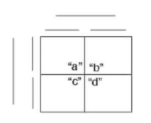
In an unbiased research study, we should expect that all possible responses are equally as likely to occur. We call this the unbiased null hypothesis and state this in terms of frequencies of responses. We can use these letters within each box to state the null hypothesis as follows:
[latex]H_{0}: f_{a} = f_{b} = f_{c} = f_{d}[/latex]
An annotated application of the 2 x 2 Chi-square to test for association between two variables
Consider a chi-square design to evaluate the relationship between maternal education and breastfeeding duration. To begin, we label the row and column headings within a fourfold table. In this example, we will use the row headings to represent the categories of maternal education and the column headings will be used to organize the breastfeeding duration as shown below in Figure 19.2.
Figure 19.2 Organization of data for 2 x 2 Chi-Square Test
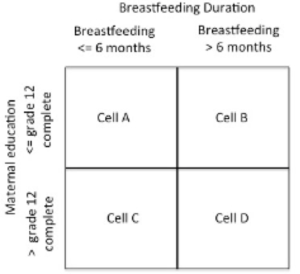
The data in Cell A represent the observation of the number of mothers who have an education level equal to or less than grade 12 and breastfed their most recent child less than 6 months. In Cell B the data represent the observation of the number of mothers who have an education level equal to or less than grade 12 and breastfed their most recent child for more than 6 months. In Cell C the data represent the observation of the number of mothers who have an education level higher than grade 12 and breastfed their most recent child less than 6 months, and in Cell D the data represent the observation of the number of mothers who have an education level higher than grade 12 and breastfed their most recent child more than 6 months.
The null hypothesis for the chi-square test of association assumes that there is no association between the variables used in the two-way table. In the example presented here, this translates to stating that there is no association between the mothers’ level of education and breastfeeding duration. In other words, breastfeeding duration does not vary in relation to the level of maternal education.
The following is an example of the application of the chi-square test of the association between breastfeeding duration and level of maternal education.
The data for 125 new mothers surveyed for breastfeeding duration and their highest level of education is shown in the following abbreviated table. The actual total observed scores for each condition of breastfeeding duration and the highest level of maternal education are provided in the table below.
Table 19.1 Abbreviated table showing breastfeeding duration and the highest level of mothers’ education for a sample of 125 new mothers.
| Subject ID | Breastfeeding duration in Months | Highest level of Maternal Education |
| 01 | 2 months | Grade 9 |
| 02 | 4 months | College complete |
| 03 | 9 months | Masters Complete |
| … | … | … |
| 123 | 18 months | Grade 11 |
| 124 | 3 months | Grade 12 |
| 125 | < 1 month | Ph.D. |
Table 19.2 The observed counts of breastfeeding duration and the highest level of mothers’ education for a sample of 125 new mothers arranged in the fourfold table
| BF duration
<= 6 months |
BF duration
> 6 months |
Row Totals | |
| Education
<= grade 12 |
Observed = 43 | Observed = 27 | n1.=70 |
| Education
> grade 12 |
Observed = 21 | Observed = 34 | n2.=55 |
| Column Totals | n.1=64 | n.2=61 | Grand Total
N=125 |
Once we have organized the observed data according to the appropriate marginal conditions, we next compute the expected values for each cell independently in the fourfold table. To compute the expected frequency independently for each cell we use the following formula:
[latex]\textit{Expected Scores} = {{\Sigma(\textit{Row frequency}}) \times {\Sigma(\textit{Column frequency}})\over \textit{Grand Total (N)}}[/latex]
Notice this formula computes the expected cell frequencies by first calculating the cross-product of the row sum multiplied by the column sum and dividing by the total sample size. The expected values in each cell are computed in Table 19.3 below.
Table 19.3 Computations of Expected Values in the 2 x 2 table
| BF duration
<= 6 months |
BF duration
> 6 months |
Row Totals | |
| Education
<= grade 12 |
Obs = 43
Exp = (70 x 64)/125 Exp = 35.84 |
Obs = 27
Exp = (70 x 61)/125 Exp = 34.16 |
n1.=70 |
| Education
> grade 12 |
Obs = 21
Exp = (55 x 64)/125 Exp = 28.16 |
Obs = 34
Exp = (55 x 61)/125 Exp = 26.84 |
n2.=55 |
| Column Totals | n.1=64 | n.2=61 | Grand Total
N observed =125 |
After calculating the expected cell values, we next compute the elements of the chi-square test for each cell of the 2 x 2 table, as follows:
STEP 1: Compute the difference between the observed and expected cell differences, then square this value and divide by the expected value within the cell.
a) in Cell A we compute: (43-35.84)2 ÷ 35.84 = 1.43
b) in Cell B we compute: (27-34.16)2 ÷ 34.16 = 1.5
c) in Cell C we compute: (21-28.16)2 ÷ 28.16 = 1.82
d) in Cell D we compute: (34-26.84)2÷ 26.84 = 1.91
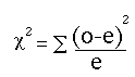
STEP 2: Sum the values computed in STEP 1 for cell A, B, C, D, above. This is the chi-square statistic. [latex]{\chi^2} ={{\Sigma(\textit{observed - expected)}^2}\over \textit{expected}}[/latex]
[latex]{\chi^2} =[/latex] = (1.43 + 1.5 + 1.82 + 1.91)
[latex]{\chi^2} =[/latex] = 6.66
STEP 3: Compare the chi-square statistic observed for this sample of data ([latex]{\chi^2}_\textit{observed} =[/latex] = 6.66) against the chi-square critical value ([latex]{\chi^2}_\textit{critical} =[/latex] = 3.84) of χ2critical =3.84. The critical value represents the chi-square statistic expected for a 2 x 2 table at a probability level of p<0.05.
STEP 4: Decision Rule: If the [latex]{\chi^2}_\textit{observed} [/latex] > [latex]{\chi^2}_\textit{critical}[/latex] then we reject the null hypothesis.
In our example, we observed that the chi-square was 6.66 which is greater than 3.84 and therefore we reject the null hypothesis that
[latex]H_{0}: f_{(j)} \textit{observed} = f_{(j)}\textit{expected}[/latex] and suggest that there is a relationship between breastfeeding duration and mother’s level of education.
Alternatively we could compute the chi-square statistic for the fourfold table using the following formula:
[latex]{\chi^2}_\textit{observed} ={ (ad-bc)^2 \times (a + b + c + d)\over{ (a+b)(c+d)(b+d)(a+c) }}[/latex]
In which case our estimate would be:
[latex]{\chi^2}_\textit{observed} ={ (43 \times 34 - 27 \times 21)^2 \times (43 + 27 + 21 +34)\over{ (43+27)(21+34)(27+34)(43+21) }}[/latex]
[latex]{\chi^2}_\textit{observed} ={ (1462 - 567)^2 \times (125)\over{ (70)(55)(61)(64) }}[/latex]
[latex]{\chi^2}_\textit{observed} ={ (100128125)\over{ (15030400) }}[/latex]
[latex]{\chi^2}_\textit{observed} = 6.66[/latex]
In the chi-square test statistic shown here, we were interested in measuring the association between breastfeeding duration and mother’s level of education completed. This is not a causal model but a measure of association that lets us evaluate the relationship between two independent measures. We began with the null hypothesis that there was no association between the two variables, but after testing the association with the chi-square test, our conclusion is that there appears to be a relationship between maternal education and breastfeeding duration.
2 x 2 CHI SQUARE WEBULATOR
Using the Chi-square Webulator[1], you can enter the data from the table above into the webulator below to compute the Chi-square observed score.
Enter the scores for cell “a” = 43, cell “b” = 27, cell “c” = 21, cell “d” = 34, and then click the buttons in the webulator to work through the calculations of the chi-square.
We can use SAS to confirm the calculations from the Webulator above.
SAS Program for the 2 x 2 chi-square:
DATA CHISQR01;TITLE '2 X 2 TABLE';INPUT ROW COL OUTCOME;/* NOTE DATA ARE ENTERED USING ROW-COLUMN ARRANGEMENT */DATALINES;1 1 431 2 272 1 212 2 34;PROC FREQ ORDER=DATA; WEIGHT OUTCOME;TABLES ROW*COL/ CHISQ EXPECTED;RUN;In the program above we use PROC FREQ with the TABLES keyword as the basic procedural statement. The TABLES statement requires the names of the row and column variables which we called ROW and COL in our example (not very imaginative!). Including the options, CHISQ and EXPECTED statements enable us to produce the statistical output for the chi-square as shown below. The other two important statements here are ORDER+DATA which maintains the position of the order in which the data were presented, respecting the row X column organization; and the keyword statement WEIGHT OUTCOME; which acknowledges that the data are not single scores but represent the sum of counts for the respective table cell. In the present example cell A: 43, Cell B: 27, Cell C: 21, Cell D: 34.
In the following output from the SAS program, both the chi-square value and the related p-value are the same as that which we calculated by hand — chi-square score = 6.66 with a p-value of <0.001. We can then make a decision to reject the null hypothesis that the count in Cell A = the count in Cell B = the count in Cell C = the count in Cell D.
Table 19.4 Results of the SAS PROC FREQ Procedure
| BF duration <= 6 months | BF duration > 6 months | Row Totals | |
| Row 1 |
Frequency = 43 Expected Freq = 35.84 Percent = 34.40 Row Pct = 61.43 Column Pct = 67.19 |
Frequency = 27 Expected Freq = 34.16 Percent = 21.60 Row Pct = 38.57 Column Pct = 44.26 |
Row 1 Total = 70 |
| Row 2 |
Frequency = 21 Expected Freq = 28.16 Percent = 16.80 Row Pct = 38.18 Column Pct = 32.81 |
Frequency = 34 Expected Freq = 26.84 Percent = 27.20 Row Pct = 61.82 Column Pct = 55.74 |
Row 2 Total = 55 |
| Column Totals | Column Total = 64
Column Pct = 51.20 |
Column Total = 61
Column Pct = 48.80 |
Grand Total = 125 |
Table 19.5 Statistics for Table of ROW by COL
| Statistic | DF | Value | Prob |
| Chi-Square | 1 | 6.6617 | 0.0099 |
| Likelihood Ratio Chi-Square | 1 | 6.7197 | 0.0095 |
| Continuity Adj. Chi-Square | 1 | 5.7638 | 0.0164 |
| Mantel-Haenszel Chi-Square | 1 | 6.6084 | 0.0101 |
| Phi Coefficient | 0.2309 | ||
| Contingency Coefficient | 0.2249 | ||
| Cramer’s V | 0.2309 |
The Case for COVID-19 Testing
One important discussion in the midst of the COVID-19 Pandemic has been related to testing. The President of the United States followed the ill-logic that by doing more testing we will naturally see a rise in the number of reported cases-full stop! Meaning that if we stick our head in the sand — aka stop testing, then we won’t see any cases. The number of problems associated with this kind of thinking is far too numerous to even begin debating the comment. However, the more important issue is, how do we use statistics to show the importance of the difference in the proportion of positive cases to all of those tested each week?
By using a 2 x 2 chi-square approach we can evaluate the significance of the changes in the proportionality between positive cases emerging from week to week. Consider the following scenario of data collection (testing and case identification) between two different weeks. Let’s say that in week 1 there were 100 tests administered, and an incidence of 35 positive cases. Next, in week 2 there were 200 cases and an incidence of 110 positive cases.
Our first step is to arrange the data collection table as shown below with Outcome (Columns) by Weeks (Rows).
| Positive Case | Negative Case | ||
| Week 1 | Cell a: 35 | Cell b: 65 | 100 |
| Week 2 | Cell c: 110 | Cell d: 90 | 200 |
| 145 | 155 | 300 |
We can use the 2 x 2 webulator to compute the chi-square statistic to determine if there is a significant difference in the proportion of cases from week 1 to week 2. Simply substitute the data from the table above into the webulator above.
Figure 19.3 First Form of the 2 x 2 Webulator
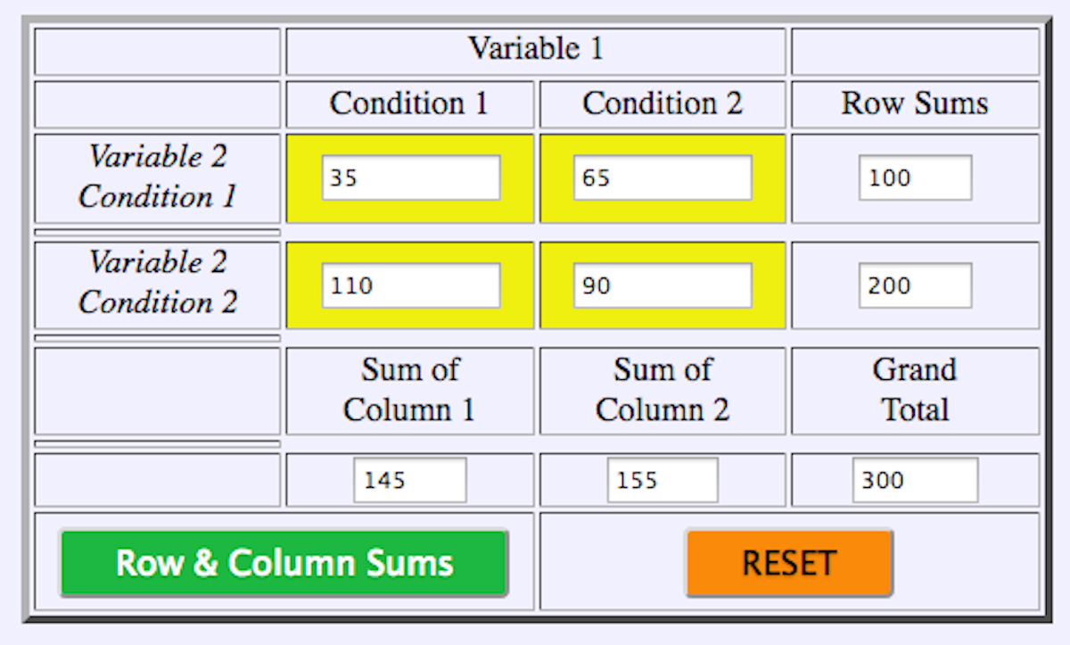
Figure 19.4 Second Form of the 2 x 2 Webulator
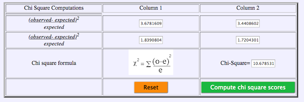
As you can see the results of the chi-square statistic observed = 10.68 which is > chi-square critical of 3.84 means that there was a significant difference between the proportions. Next, we can compare these data using SAS as shown below.
Chi-square for COVID-19 cases versus tests
DATA COVIDCHI;
TITLE ‘COVID – 19 CHISQUARE 2 X 2 TABLE’;
INPUT ROW COL OUTCOME;
/* NOTE DATA ARE ENTERED USING ROW-COLUMN ARRANGEMENT */
DATALINES;
1 1 35
1 2 65
2 1 110
2 2 90
;
PROC FREQ ORDER=DATA; WEIGHT OUTCOME;
TABLES ROW*COL/ CHISQ EXPECTED;
RUN;
TITLE ‘COVID – 19 CHISQUARE 2 X 2 TABLE’;
INPUT ROW COL OUTCOME;
/* NOTE DATA ARE ENTERED USING ROW-COLUMN ARRANGEMENT */
DATALINES;
1 1 35
1 2 65
2 1 110
2 2 90
;
PROC FREQ ORDER=DATA; WEIGHT OUTCOME;
TABLES ROW*COL/ CHISQ EXPECTED;
RUN;
Table 19.6 Statistics for Table of ROW by COL
From these data, we observe that regardless of the number of tests administered, the estimate of interest is not merely the number of tests conducted but the proportionality of the number of positive tests from one week to the next.
- <script src="https://pressbooks.library.upei.ca/montelpare/wp-content/plugins/h5p/h5p-php-library/js/h5p-resizer.js" charset="UTF-8"></script> ↵
