
| RATIO | P1 | P2 | RELRISK | M1 | M2 | M | TOTALN |
|---|---|---|---|---|---|---|---|
| 0.5 | 0.01 | 0.015 | 1.5 | 11307.92 | 11907.92 | 11908 | 17862.0 |
| 0.5 | 0.01 | 0.020 | 2.0 | 3316.17 | 3616.17 | 3617 | 5425.5 |
| 0.5 | 0.01 | 0.030 | 3.0 | 1070.02 | 1220.02 | 1221 | 1831.5 |
| 0.5 | 0.05 | 0.075 | 1.5 | 2148.71 | 2268.71 | 2269 | 3403.5 |
| 0.5 | 0.05 | 0.100 | 2.0 | 623.23 | 683.23 | 684 | 1026.0 |
| 0.5 | 0.05 | 0.150 | 3.0 | 196.32 | 226.32 | 227 | 340.5 |
| 0.5 | 0.10 | 0.150 | 1.5 | 1003.79 | 1063.79 | 1064 | 1596.0 |
| 0.5 | 0.10 | 0.200 | 2.0 | 286.59 | 316.59 | 317 | 475.5 |
| 0.5 | 0.10 | 0.300 | 3.0 | 87.07 | 102.07 | 103 | 154.5 |
| 0.5 | 0.20 | 0.300 | 1.5 | 431.30 | 461.30 | 462 | 693.0 |
| 0.5 | 0.20 | 0.400 | 2.0 | 118.21 | 133.21 | 134 | 201.0 |
| 0.5 | 0.20 | 0.600 | 3.0 | 32.31 | 39.81 | 40 | 60.0 |
| 0.5 | 0.43 | 0.645 | 1.5 | 124.93 | 138.88 | 139 | 208.5 |
| 0.5 | 0.43 | 0.860 | 2.0 | 27.76 | 34.74 | 35 | 52.5 |
| 0.5 | 0.43 | 1.290 | 3.0 | . | . | . | . |
| 1.0 | 0.01 | 0.015 | 1.5 | 7749.59 | 8149.59 | 8150 | 16300.0 |
| 1.0 | 0.01 | 0.020 | 2.0 | 2318.16 | 2518.16 | 2519 | 5038.0 |
| 1.0 | 0.01 | 0.030 | 3.0 | 768.01 | 868.01 | 869 | 1738.0 |
| 1.0 | 0.05 | 0.075 | 1.5 | 1470.49 | 1550.49 | 1551 | 3102.0 |
| 1.0 | 0.05 | 0.100 | 2.0 | 434.43 | 474.43 | 475 | 950.0 |
| 1.0 | 0.05 | 0.150 | 3.0 | 140.10 | 160.10 | 161 | 322.0 |
| 1.0 | 0.10 | 0.150 | 1.5 | 685.60 | 725.60 | 726 | 1452.0 |
| 1.0 | 0.10 | 0.200 | 2.0 | 198.96 | 218.96 | 219 | 438.0 |
| 1.0 | 0.10 | 0.300 | 3.0 | 61.60 | 71.60 | 72 | 144.0 |
| 1.0 | 0.20 | 0.300 | 1.5 | 293.15 | 313.15 | 314 | 628.0 |
| 1.0 | 0.20 | 0.400 | 2.0 | 81.22 | 91.22 | 92 | 184.0 |
| 1.0 | 0.20 | 0.600 | 3.0 | 22.33 | 27.33 | 28 | 56.0 |
| 1.0 | 0.43 | 0.645 | 1.5 | 83.23 | 92.53 | 93 | 186.0 |
| 1.0 | 0.43 | 0.860 | 2.0 | 18.21 | 22.87 | 23 | 46.0 |
| 1.0 | 0.43 | 1.290 | 3.0 | . | . | . | . |
| 5.0 | 0.01 | 0.015 | 1.5 | 4876.35 | 5116.35 | 5117 | 30702.0 |
| 5.0 | 0.01 | 0.020 | 2.0 | 1497.47 | 1617.47 | 1618 | 9708.0 |
| 5.0 | 0.01 | 0.030 | 3.0 | 509.46 | 569.46 | 570 | 3420.0 |
| 5.0 | 0.05 | 0.075 | 1.5 | 922.50 | 970.50 | 971 | 5826.0 |
| 5.0 | 0.05 | 0.100 | 2.0 | 278.84 | 302.84 | 303 | 1818.0 |
| 5.0 | 0.05 | 0.150 | 3.0 | 91.63 | 103.63 | 104 | 624.0 |
| 5.0 | 0.10 | 0.150 | 1.5 | 428.25 | 452.25 | 453 | 2718.0 |
| 5.0 | 0.10 | 0.200 | 2.0 | 126.50 | 138.50 | 139 | 834.0 |
| 5.0 | 0.10 | 0.300 | 3.0 | 39.39 | 45.39 | 46 | 276.0 |
| 5.0 | 0.20 | 0.300 | 1.5 | 181.10 | 193.10 | 194 | 1164.0 |
| 5.0 | 0.20 | 0.400 | 2.0 | 50.30 | 56.30 | 57 | 342.0 |
| 5.0 | 0.20 | 0.600 | 3.0 | 13.23 | 16.23 | 17 | 102.0 |
| 5.0 | 0.43 | 0.645 | 1.5 | 48.78 | 54.36 | 55 | 330.0 |
| 5.0 | 0.43 | 0.860 | 2.0 | 9.33 | 12.12 | 13 | 78.0 |
| 5.0 | 0.43 | 1.290 | 3.0 | . | . | . | . |
| 20.0 | 0.01 | 0.015 | 1.5 | 4330.01 | 4540.01 | 4541 | 95361.0 |
| 20.0 | 0.01 | 0.020 | 2.0 | 1337.06 | 1442.06 | 1443 | 30303.0 |
| 20.0 | 0.01 | 0.030 | 3.0 | 455.75 | 508.25 | 509 | 10689.0 |
| 20.0 | 0.05 | 0.075 | 1.5 | 818.22 | 860.22 | 861 | 18081.0 |
| 20.0 | 0.05 | 0.100 | 2.0 | 248.38 | 269.38 | 270 | 5670.0 |
| 20.0 | 0.05 | 0.150 | 3.0 | 81.54 | 92.04 | 93 | 1953.0 |
| 20.0 | 0.10 | 0.150 | 1.5 | 379.23 | 400.23 | 401 | 8421.0 |
| 20.0 | 0.10 | 0.200 | 2.0 | 112.27 | 122.77 | 123 | 2583.0 |
| 20.0 | 0.10 | 0.300 | 3.0 | 34.73 | 39.98 | 40 | 840.0 |
| 20.0 | 0.20 | 0.300 | 1.5 | 159.68 | 170.18 | 171 | 3591.0 |
| 20.0 | 0.20 | 0.400 | 2.0 | 44.15 | 49.40 | 50 | 1050.0 |
| 20.0 | 0.20 | 0.600 | 3.0 | 11.22 | 13.85 | 14 | 294.0 |
| 20.0 | 0.43 | 0.645 | 1.5 | 42.00 | 46.88 | 47 | 987.0 |
| 20.0 | 0.43 | 0.860 | 2.0 | 7.26 | 9.71 | 10 | 210.0 |
| 20.0 | 0.43 | 1.290 | 3.0 | . | . | . | . |
Advanced Concepts for Applied Statistics in Healthcare
41 Using Webulator Applications to Compute Sample Size
In this chapter, we will work through four different approaches to sample size calculations using bespoke Webulators based on probabilistic formulae.
1. Determining Sample Size for a Simple Random Sample to Estimate a Population Proportion
Elements of the Webulator and Sample Size for a Population Proportion
The sample size formula for a population proportion is based on the formula shown here.
Figure 41.1. Formula to Determine Sample Size for a Population Proportion
Unpacking the formula for simple random sampling we see that N represents the population from which the sample will be drawn; the proportion (p) refers to the proportion of individuals displaying the characteristic of interest, while (1-p) or (q) refers to the proportion of individuals in the population not displaying the characteristic of interest.
To determine the proportion of cases in a population, p is the ratio of all individuals displaying the characteristic of interest divided by the set of all cases from which the sample was drawn. In real life, you might determine p based on past research or population statistical data such as the census.
The error term in the denominator refers to the expected accuracy or the allowable difference between the estimate of the proportion in the selected sample, as a result of the sample size calculation, and the true population proportion. A typical value here would range between 0.02 and 0.10.
The term refers to the two-tailed standardized score of researcher confidence. If =0.05 then z= 1- = 0.95 or a 95% confidence value.
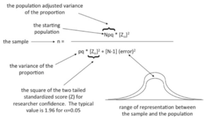
Figure 41.2. Explaining the parts of the formula
Application of the Sample Size Formula for a Population Proportion
Using the Webulator for a Population Proportion you can produce a representative sample for the population based on a simple random sampling approach. Consider that you are asked by the Chief Public Health Officer (CPHO) to determine the sample size required to represent a proportion of persons who inject drugs (PWID) based on a starting population of 157,000 individuals. From previous reports, the proportion of PWID within a sample (i.e. the proportion of the population that displays the characteristic of interest) was about 13% or p = 0.13 and therefore q = (1-p) = 0.87. The CPHO wants the estimate to be within 3% of the true population proportion with 95% confidence. Below is a Webulator to calculate the sample size for this scenario – i.e. a population proportion.
Follow these basic steps to use this webulator to compute the sample size for this scenario, or any situation where you need to determine the sample size for a population proportion.
- Enter 157000 into the Webulator in the field labelled Initial Population
- Next, enter 0.13 of 13 into the Webulator in the field labelled Expected Proportion
- Enter 1.96 into the field labelled Zalpha for the percent confidence, as this is the corresponding z-score for 95% confidence
- Finally, enter the number 3 into the Webulator in the field labelled Percent Error
- Click the button labelled calculate.
Based on the application of the formula for simple random sampling for the estimate of a Population Proportion you report that the CPHO will require a sample size of at least 481 individuals in order to be 95% confident that the proportion of PWID in her sample will represent the true population proportion of PWID individuals within 3%.
2. Determining Sample Size for a Comparison Study
In some research designs, we are interested in comparing results between two or more groups. In this case, we may not know the original population size, but we may know about variability with respect to the dependent variables. To determine the sample size for a comparison study we need to know the measure of central tendency for the dependent variable and the amount of variability we could expect for the measures of the dependent variable.
Typically, the amount of variability is based on information from previous studies. In some situations, this information may come from pilot work or from an actual study. The sample size formula for comparison studies is shown here as:
Figure 41.2 Formula to Determine Sample Size for a Population Proportion
The [Zalpha ] and [Zbeta] terms are provided in the following tables. The area under the normal curve for the [Zbeta] term is illustrated in the Figure 41.3
Figure 41.3 Areas under the Normal Curve representing [latex]z_{beta}[/latex] scores
The terms of the formula are explained as follows. The term is based on the variance reported in the literature or from pilot studies. Similarly, the expected mean is based on the mean from the literature or from pilot studies, while the expected % accuracy is the proximity of the estimated mean score to the true population score and is set by the researcher to be about 10%. The terms Zalpha or Zand Zbeta or Z use the standard scores for the alpha level and for the beta value (power) levels. Common values for and are =0.05 and =1.28, respectively. A more comprehensive table of conversions of areas under the normal curve representing [latex]z_{alpha}[/latex] and [latex]z_{beta}[/latex] scores are shown in Tables 41.2 and 41.3, below.
| Table 41.2 Conversion table to create the Z beta term |
| (one tailed probability estimate=0.05); beta = 0.10 (power = 90%) ; [Zbeta] = 1.64 |
(one tailed probability estimate=0.06); beta = 0.12 (power = 88%) ; [Zbeta] = 1.55 |
| (one tailed probability estimate=0.07); beta = 0.14 (power = 86%) ; [Zbeta] = 1.48 |
(one tailed probability estimate=0.08); beta = 0.16 (power = 84%) ; [Zbeta] = 1.41 |
| (one tailed probability estimate=0.09); beta = 0.18 (power = 82%) ; [Zbeta] = 1.34 |
(one tailed probability estimate=0.10); beta = 0.20 (power = 80%) ; [Zbeta] = 1.28 |
| Table 41.3 Conversion table for alpha and percent confidence to Z |
| (alpha probability estimate of 0.10)=90% [Zalpha] = 1.64 |
(alpha probability estimate of 0.09)=91% [Zalpha] = 1.70 |
| (alpha probability estimate of 0.08)=92% [Zalpha] = 1.75 |
(alpha probability estimate of 0.07)=93% [Zalpha] = 1.81 |
| (alpha probability estimate of 0.06)=94% [Zalpha] = 1.88 |
(alpha probability estimate of 0.05)=95% [Zalpha] = 1.96 |
| (alpha probability estimate of 0.04)=96% [Zalpha] = 2.05 |
(alpha probability estimate of 0.03)=97% [Zalpha] = 2.17 |
| (alpha probability estimate of 0.02)=98% [Zalpha] = 2.33 |
(alpha probability estimate of 0.01)=99% [Zalpha] = 2.58 |
Application of the Sample Size Formula for a Comparison Study
In a recent healthy heart study, researchers measured the effects of red wine consumption on blood cholesterol concentrations of males over the age of 35 years. The researchers showed that males (n1= 133) who consumed on average one serving of red wine per day, for a minimum of six days per week, had a lower concentration of the athero-genic low-density lipoprotein cholesterol than a group of age-matched control subjects (n2= 143) who abstained from any alcohol consumption. The investigation followed the total group of 276 males for a 24 week period.
You believe that the data are valuable and therefore you wish to conduct the study with a group of males in your local community. In the reference study, the average cholesterol concentration for the sample of interest (red wine consumers) was 4.6 mmol/L with a standard deviation of 0.32 millimoles per litre (mmol/L). Considering that you wish to use an alpha level of 0.05 with a corresponding beta level of 4 x alpha (where beta = 4 x 0.05 = 0.20) and a power level of “1 – beta = 0.80”. Further, you expect that the difference between your estimate of the mean and the TRUE estimate of the mean is within 3 percent.
Using the Webulator for a Comparison Study you can produce a representative sample for the population based on a simple random sampling approach. The data you need in order to compute the appropriate sample size is:
- The estimated mean from previous studies = 4.6 mmol/L
- The standard deviation from previous studies = 0.32
- The z scores for the alpha probability (.05), Zα=1.96
- The z score for the beta probability (.20), Zβ=1.28
- The allowable percent difference between your estimate for the dependent variable and the expected estimate for the dependent variable from the true population = 3%
The results of this computation indicate that in order to be 95% confident that the estimates for the proposed sample will be within 3 percent of the true population value, you will need to have a minimum of 16 participants in the test group and 16 participants in the control group.
3. Determining Sample Size for a Case-Control Study
In the case-control study design, individuals with a specific measurable condition are “compared” to individuals that do not demonstrate the condition of interest. The case-control design is a retrospective study design type that evaluates, by comparison, the differences in outcome measures between groups of individuals with and without a disease, or the signs/symptoms of a condition.
Case-control studies are useful in demonstrating associations but may not show causation. The temporal characteristics (elements of time) are important in demonstrating the relationship. An essential consideration in a case-control study is the clear definition of the cases and of the controls.
In a case-control design we may also consider that the cases are more likely to occur given exposure to the stimulus, to which we say this is a directional hypothesis or a one-tailed hypothesis. If we consider a one-tailed decision rule (cases are more likely than controls, given the characteristics of the scenario) then we see that a power of 80% has a beta term of 0.20 and a Zβ= 0.084. Estimates of statistical power for the one-tailed (directional hypothesis) and corresponding Zβ values are shown in the following table.
Table 41.5 Power estimates from the [latex]z_{beta}[/latex] terms in a one-tailed hypothesis
| POWER | [latex]z_{beta}[/latex] |
| 80% | 0.84 |
| 85% | 1.04 |
| 90% | 1.28 |
| 95% | 1.64 |
The sample size formula to determine the number of cases (or the number of controls) in each group of a case-control study is shown here as:
Figure 41.4. Formula to Determine Sample Size for a Case-Control Application
The formula differs slightly from that published more recently by Kasiulevicius, Sapoka, and Filipaviciute (2006)[1] but produces similar estimates. Where the elements of the formula include: the proportion of cases among those individuals suspected to have been exposed. : the proportion of cases among those individuals suspected to not have been exposed. : is the Z score for the term, where 1.96, and: is the Z score for the term for a one-tailed directional hypothesis ( 0.84).
Application of the sample size formula for a case-control study
In order to determine the effects of cannabis smoking on lung cancer you decide to conduct a retrospective case control study in which your sample size estimate is based on the consideration that the relative risk of lung cancer among frequent cannabis smokers is about 5.7 times that of non-smokers. You decide to use p1 = 0.285 to represent the proportion lung cancer patients who were frequent cannabis smokers and p0 = 0.05 to represent the proportion lung cancer patients as controls who never smoked cannabis.
The data needed to compute the appropriate sample size are shown here as:
- Proportion of individuals that had lung cancer among individuals that were considered frequent smokers of cannabis, P1 = 0.285
- Proportion of individuals that had lung cancer among individuals that never smoked cannabis, P0 = 0.05
- The z scores for the alpha term (α=0.05), Zα=1.96
- The z scores for the beta term based on a one-tailed hypothesis, [latex]z_{beta}[/latex] =0.84
As you can see in the results of the computation using the Webulator the appropriate sample size needed to conduct your study will require at least 36 individuals in the case group and at least 36 individuals in the control group.
4. Determining Sample Size for a Cohort Comparison Study
As described previously, the cohort comparison study design is a type of observational study in which the researcher simply observes an outcome without intervening. As a longitudinal study design, the cohort study design follows a group of individuals with similar characteristics either forward in time (prospectively) or backward in time (retrospectively).
In the cohort comparison study design a group demonstrating the characteristic(s) of interest are followed for a period of time while being compared to a similar group or multiple similar comparison groups (the cohorts) that do not demonstrate the characteristic(s) of interest. The researcher is intending to measure specific variables within the designated cohort of interest and to compare such measures to those reported for the comparison cohort(s). Throughout the monitoring stage, the selected measures are recorded at the onset of the monitoring activity, at pre-designated time points throughout the study, and at the completion of the study.
The formula to compute the sample size for the group of interest in a cohort comparison study where the data are normally distributed is shown here:
[latex]n ={ \left[ Z_\alpha \sqrt{ (1+{\left(1\over{m}\right)} ) \times{\left(\overline{p} (1-{\overline{p}})\right) }} + Z_\beta\sqrt{{p_0(1-p_0)\over{m}} + p_1 (1-p_1)}\right]^2 \over{(p_0 - p_1)^2} }[/latex]
The essential elements required for the computation of sample sizeinclude:
The sample size computations are based on Fleiss (1981). The following SAS program was originally written by Dr. P.N. Corey (University of Toronto) and includes a continuity correction that was not included in Fleiss’ original calculations. This SAS program uses a probit function to enable the input of any alpha and beta values.
* PROGRAM NAME IS SScohort.SAS ;
OPTIONS PS = 65 LS = 80 NODATE NONUMBER ;
TITLE1 ‘SAMPLE SIZE DETERMINATION USING THE FORMULAE FROM Fleiss 1981’;
************************************************************
** Program SAMPSIZEFLEISSA.SAS has been modified to allow **
** DO LOOPS to be defined in %LET statements outside the **
** body of the program and calculates sample sizes N1 = m **
** and N2 = rm for a cohort or cross-sectional study that **
** involves the comparison of two independent samples **
** using a correction factor for continuity. The program **
** makes a small modification to the program SAMPSIZE2.FLS**
** by defining PBAR differently. **
************************************************************;
********* PARAMETER DEFINITION USING %LET STATEMENT ********;
%LET ALPHA = 0.05 ;
%LET BETA = 0.20 ;
%LET RATIOLIST = 0.50, 1.0, 5.0, 20.0;
%LET P1LIST = 0.01, 0.05, 0.10, 0.2, 0.43;
%LET RRLIST = 1.5, 2, 3 ;
************************************************************
* If we use the DO LOOP DO RATIO = (1/2),1,2 we would be *
* asking the program to estimate the sample sizes for the *
* following situations *
* (a) N1 is one half the number N2 *
* (b) N1 is equal to N2 *
* (c) N1 is twice the size of N2 *
************************************************************;
************************************************************
* If we use the DO LOOP DO P1 = 0.10, 0.20 we would be *
* asking the program to estimate the sample sizes for the *
* following situations *
* (a) P1 = 0.10 *
* (b) P1 = 0.20 *
************************************************************;
************************************************************
* If we use the Do LOOP DO RELRISK = 2 to 4 we would be *
* asking the program to estimate the sample sizes for the *
* following situations *
* (a) P2 is twice the size of P1 *
* (b) P2 is three times the size of P1 *
* (c) P2 is four times the size of P1 *
************************************************************;
********** NO CHANGES BEYOND THIS POINT IN PROGRAM *********;
DATA TEMP1 ;
ALPHA = 0 + &ALPHA ;
BETA = 0 + &BETA ;
DO RATIO = &RATIOLIST ; ***<<<— See explanation above ***;
DO P1 = &P1LIST ; ***<<<— See explanation above ***;
DO RELRISK = &RRLIST ; ***<<<— See explanation above ***;
POWER = 1 – &BETA ;
ZALPHA = PROBIT((1 – &ALPHA/2));
ZBETA = PROBIT((1 – &BETA)) ;
P2 = RELRISK * P1 ; Q1 = 1 – P1 ; Q2 = 1 – P2 ; DELTA = P2 – P1 ;
PBAR = (P1 + RATIO * P2 ) / (RATIO + 1) ; QBAR = 1 – PBAR ;
NUMERAT1 = ZALPHA * SQRT((RATIO + 1) * PBAR*QBAR) +
ZBETA * SQRT(RATIO*P1*Q1 + P2*Q2) ;
M1 = ((NUMERAT1/DELTA)**2) / RATIO ;
M2 = M1 + (RATIO + 1)/(RATIO * ABS(P2 – P1)) ; M = INT(M2 + 1) ;
TOTALN = M + RATIO * M ;
OUTPUT ; END ; END ; END ;
PROC PRINT DOUBLE NOOBS ;
VAR RATIO P1 P2 RELRISK M1 M2 M TOTALN ;
TITLE1 ‘SAMPLE SIZE DETERMINATION USING THE FORMULAE FROM THE BOOK’;
TITLE2 ‘STATISTICAL METHODS FOR RATES AND PROPORTIONS’ ;
TITLE3 ‘BY JOSEPH L. FLEISS SECOND EDITION JOHN WILEY AND SONS’ ;
TITLE4 “FOR TYPE I ERROR RATE &ALPHA AND TYPE II ERROR RATE &BETA”;
RUN ;
The output generated by the SScohort.sas program is shown below.
