
III. ASSEMBLING THE VISUAL IMAGE
27. HOLISTIC IMAGING
There is a way to transform images that is even more efficient than into lines. Transforming images into spatial frequencies requires even fewer channels to transmit them and facilitates calculations such as adding and comparing images. Subsequent reverse transformation restores the original or produces a new image that results from calculations. This is similar to how logarithms work.[1]
Appendix H – Spatial Frequencies shows how spatial frequency waves can be combined (Fourier synthesized) to produce definite shapes. It is a reverse explanation of how shapes can be broken down (Fourier analyzed) into spatial frequencies. These transformations are the most efficient means known for transmitting and processing images. That efficiency led to their use in animal neural networks early in the evolution of visual systems.
Is there evidence that our visual system actually does this?
To start, the structure of our eyes makes them more sensitive to spatial frequencies around 3 cycles per degree than higher and lower ones.
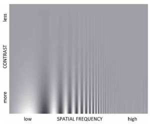 See for yourself:
This figure cascades a range of spatial frequencies horizontally, while continuously decreasing the contrast vertically.
Seeing the modulations higher up indicates greater sensitivity to that spatial frequency.
Note your decrease in contrast sensitivity at the low and high frequencies. The need for more contrast to see fine details is evident in everyday experience. That large features in an image also require more contrast may surprise you.
In 1969, Colin Blakemore & Fergus Campbell reported an experiment that used the selective adaptation method (page 111) to measure visual sensitivity to spatial frequency patterns. They found clear evidence of neural channels selectively tuned to various spatial frequencies in human vision. [2]
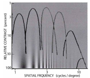 Here representations of the spatial-frequency tuning curves are laid over the above spatial frequency sensitivity demonstration:
This is the basis of how the visual system analyzes the retinal image into spatial frequencies along a single dimension.
This Fourier-like analysis makes the encoding of images more efficient than linear analysis. In turn, that facilitates their recognition, interaction with memory, and control of movement.
Six overlapping spatial frequency channels may seem too few to reproduce the subtle details of our visual image. Yet consider how:
1. Only three color receptors give us some 150 hues.
2. Seven or eight orientation tuned channels suffice to produce some hundreds of line orientations.
It’s another example of population encoding whereby a few tuned channels can code many spatial frequencies.
This selective adaptation exercise demonstrates that you have visual channels tuned to spatial frequencies:
At first glance, the gratings in the upper and lower boxes on the right look the same. Now, stare at the bar between the two boxes on the left. Move your gaze back and forth along this bar for one minute. Then, shift your gaze to the spot between the two boxes on the right. [3]
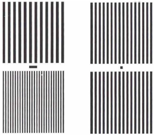
The two gratings on the right now are no longer the same. Lines in the upper grating are a bit closer together, while lines in the lower grating are a bit further apart.
This demonstration is similar to that showing visual channels for line orientation – see Part III.
Its explanation on the next page, though brief, is similar to the
explanation of orientation tuning.
Extended viewing (adaptation) of the 2.3 cycles per degree (cpd) grating depletes the resources of the neurons in that channel, weakening its response.
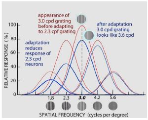 Since the 1.8, 3.0, and 4.2 cpd channels are partly sensitive to 2.3 cpd, their neural responses are also weakened.
When you then look at the 3.0 cpd grating, the composite or population encoded output of all channels thus ends up being maximal between 3.0 and 4.2 cpd. This briefly makes the 3.0 cpd grating appear to have a frequency of 3.6 cpd – though there is no channel maximally sensitive to that spatial frequency.
(Look back at Ch 25 for its more detailed explanation of how selective adaptation works.)
This is yet another example of the visual system slightly distorting visual image it creates from the optical image of the world. We rarely to stare fixedly at simple patterns. Therefore, spatial frequency tuning is a trivial risk for the sake of efficient information processing.[4]
Karl Pribram (1990) proposes that the visual system’s analysis of retinal images into spatial frequencies is followed by a synthesis back into a visual image. [5]
Here is a representation:
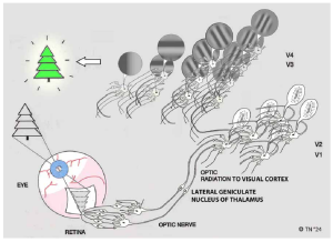 Based on Pribram’s theory, spatial frequency synthesis of the retinal image is done by a further neural network that assembles the linear receptive fields of neurons in V1 & V2 to converge on single neurons in V3 & V4, creating spatial frequency fields.
(The balloons depict the retinal image patterns to which that neuron responds to best – its receptive field.)
Images formed by the synthesis of multiple spatial frequencies at various orientations are called “holograms”. (Because spatial frequency encoding is very efficient, encoding an image from different perspectives and superimposing them is possible. That can produce the sort of 3-dimensional images popularized in movies.) Yes, they do resemble the “picture in your head”.
Holographic image processing is a type of 2nd order population encoding based on the limited number of spatial frequency and orientation tuned visual channels. A 2nd order process then synthesizes these in various combinations to form specific images. On the basis of this model, we do not have single cortical neurons tuned to flower, house or tree shapes because we do not need them any more than we need neurons tuned to orange or to lines oriented at 83 degrees.
The speculative part is what produces that “white arrow” leading to the conscious image from the activity of those spatial frequency neurons.
Still, there is more than brightness, color, and shape in visual images. We consider some of these visual processing effects in the next two sections.
- Numbers can be transformed into logarithms with a log table. To multiply two numbers, add their logarithms, then un-transform their sum using an antilog table to see the product. Dividing a logarithm by 2 and taking the antilog gives a square root. Similarly, shapes can be transformed into spatial frequencies by Fourier analysis. Adding the spatial frequency versions of several shapes and Fourier synthesizing the sum produces a composite image. ↵
- Blakemore C & Campbell FW (1969) On the existence of neurones in the human visual system selectively sensitive to the orientation and size of retinal images. Journal of Physiology, 203, 237-260. Blakemore & Campbell did not receive a Nobel Prize - unlike Hubel & Weisel. This oversight seems to be due to: 1) Many vision researchers then did not understand the significance of Fourier processing for image transmission and storage. 2) Physiological measurements are widely regarded as more “scientific” than psychophysical measurements. 3) It took several years before physiological data confirmed spatial frequency tuning in the visual cortex: Maffei L & Fiorentini A (1973) The visual cortex as a spatial frequency analyzer. Vision Res. 13, 12551267. A recent example: Altan E, Morgan C, Dakin S & Schwarzkopf DS (2024) Spatial frequency adaptation modulates population receptive field sizes. Elife, {https: doi.org/10.7554éeLife.100734}. ↵
- This figure demonstrates that our visual system has neural mechanisms that are tuned to specific spatial frequencies of bars tilted at specific angles. At first glance, the right upper and lower sets of bars look the same. After staring at the left sets of bars for a minute, the right bars are no longer the same. The upper bars have shifted to a higher spatial frequency. The lower bars have shifted to a lower spatial frequency. These shifts are in the opposite direction of how they differ from the bars on the right. Subsequent pages explain that staring at the upper bars on the left fatigued the low spatial frequency mechanisms in that part of the visual field. Their influence was then weak when viewing the bars on the right. ↵
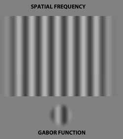
- The spatial frequency analysis and synthesis of optical holography uses waves spread across an entire image and defined by their relative location or phase as ell as frequency. An analogous process is not possible in biological visual systems based on neurons with limited visual fields. Used instead is a localized spatial frequency format - the Gabor transformation: While the number of Gabor functions needed to add up to a particular shape increases with its size, that still means several orders of magnitude fewer components than assembly from pixels or line element receptive fields.
 ↵
- Appendix H - Spatial Frequencies Pribram KH (1990) Brain and Perception. Hillsdale, N.J.: Lawrence Erlbaum Associates. Blakemore & Campbell’s discovery implies that spatial frequency analysis ought to be followed by synthesis, leading to the visual image of the world before our eyes. (Otherwise, why bother?) That synthesis is complicated by the fact that different spatial frequencies are analyzed in different areas of the visual cortex - for example: Kaufmann L, et al. (2015) Spatial frequency processing in scene-selective cortical areas. NeuroImage, 112, 86-95. How that synthesis then occurs is a Binding Problem. How that synthesis results in our visual image is a Hard Problem. Both problems will be discussed later. First, other visual processes are also involved in organizing that image. ↵