
APPENDIX H – Spatial Frequencies (Analysis and Synthesis)
Waves that vary rhythmically in intensity along a particular direction on a surface are called spatial waves. They are characterized by the number of intensity-variation cycles per unit distance – their spatial frequency. Below is a surface with spatial waves that vary only in the Y dimension:
These waves are described in terms of their number of cycles per Y-axis distance. That distance is specified in terms of angular distance with respect to the viewer – cycles per degree.
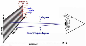
(This enables describing the fineness or coarseness of the spatial wave viewed at any distance with a single metric.)
This is a spatial frequency wave of 1 cycle/degree in the Y direction:
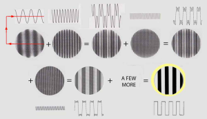
It might seem impossible to create an abrupt intensity change by adding together waves that change gradually in intensity, but it can be done. Here is a succession of surface waves whose frequency varies from left to right. When each is in a specific position or relative phase, their sum produces a surface wave with a series of rectangular changes in intensity:
 Most images of interest vary in intensity in two directions. Here, waves varying in one dimension interact with waves varying in the second dimension of a surface:
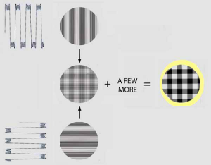
Such two-dimensional interactions of surface sinewaves represent the basis of how sine waves can combine to produce complex images. The advantage of representing a shape in terms of waves instead of lines increases exponentially in terms going from one to two dimensions in terms of the number of elements needed to reproduce the shape. It would take thousands of spots or hundreds of lines to produce the above check pattern. Just a dozen or so vertical and horizontal sine gratings would suffice.
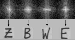 To see how adding up sine waves can produce realistic images, here some letters of the alphabet are synthesized from two-dimensional composites of sine waves: [1]
Adding sine waves together to produce any possible shape is called Fourier synthesis.
These Fourier calculations can be reversed: Any shape can broken down, i.e. Fourier analyzed, into a unique combination of spatial frequencies. (Though this Appendix seeks to explain the analysis of images into spatial frequencies, it is easier to illustrate the principle first in terms of synthesis.)
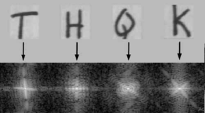
Spatial frequency processing of images is called holography. It is a holistic method of storing information in that the entire surface stores information about each image point through the inter-action of spread-out waves.
Any 2- or 3-dimensional image can be Fourier analyzed into spatial frequency waves. Here, the image of that room is analyzed into its spatial frequency components in two dimensions:
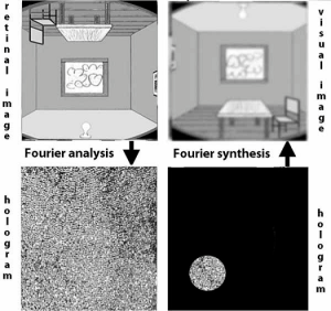
This hologram of a more complex image looks random. However, it is not. This becomes evident when just a portion of the hologram is synthesized, as shown on the right.
Note that the entire image is still there – just less sharp.
Our recall of scenes tends to fade similarly in memory. This was one of the properties of holographic processing that led Karl Pribram to propose that the visual system analyzed retinal images into spatial frequencies to transmit and store that information efficiently. [2]
Analysis of graphic images into spatial frequencies and synthesis back into graphic images is like working with logarithms: A lot of advanced math is all about transforming equations into another format that is easier to operate, doing the arithmetic, and then reverse-transforming the result back to the original format.
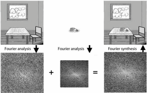
Analyzing images into spatial frequencies facilitates information processes such as adding images together:
This represents how a spatial frequency trans formation of an image of a room enables adding a transformed image of a dinner plate to put dinner on the table.
There is evidence that neural activity retrieved from memory strongly resembles the sensory response to the original image. [3]
Holographic processing would enable visual images in spatial frequency mode to be rapidly compared with memory to obtain recognition.
Such efficiency in information processing would strongly influence evolving its use for vision. Furthermore, there seems to be no other reason why the visual system would go to the trouble of breaking down the retinal image into spatial frequencies.
Here is a guide to recognizing the somewhat obscure figure in Ch 29:
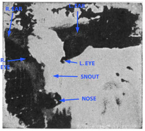
Many persons have reported that it is difficult to see the cow, but once seen, it is difficult not to see it.
- This figure is used with permission from Dr. J. Bryar’s “Introduction to Fourier Transforms of Images”, a short internet course(https://www.cs.unm.edu/~brayer/vision/fourier.html) from the University of New Mexico that provides a non-mathematical explanation of how Fourier transforms work. ↵
- Pribram KH (1990) Brain and Perception. Hillsdale, N.J.: Lawrence Erlbaum Associates. Blakemore & Campbell’s discovery implies that spatial frequency analysis ought to be followed by synthesis, leading to the visual image of the world before our eyes. (Otherwise, why bother?) That synthesis is complicated by the fact that different spatial frequencies are analyzed in different areas of the visual cortex - for example: Kaufmann L, et al. (2015) Spatial frequency processing in scene-selective cortical areas. NeuroImage, 112, 86-95. ↵
- Nilsson TH (2020) What came out of visual memory: Inferences from difference-thresholds, Attention, Perception & Psychophysics, 82, 2963-2984. ↵