
APPENDIX E – Psychophysical Methods
Much of our understanding of how the visual system processes the retinal image to produce a visual image has been gained by objectively measuring specific visual effects in terms of physical effects. This Appendix explains how that is possible.
When Benjamin Thomson sought to find out which of his lamp designs produced the most light, he found his brightness judgments were inconsistent. He was up against the same problem that hampered philosophers and scientists of his day when they sought to study the mind. There seemed to be no way to apply the quantitative methods that were so successfully advancing knowledge in physics, chemistry, and biology. Evidently being of a practical bent, especially when it came to money, Thompson forged ahead anyway and came up with a measurement method, the likes of which would take over fifty years to be discovered – again.
In 1850, Fechner realized that many subjective aspects of perception could be measured objectively. He described two aspects of perception, thresholds and difference-thresholds, and three ways to measure them in physical terms. Because they measure subjective effects in terms of physical effects, they are called “psychophysical” methods. What follows are some brief descriptions of how they work, plus an additional method developed later.
1. Threshold Measurements
We can learn much about how any “system” works by determining its operating limits or thresholds, even when more specific responses of the system can’t be directly measured. For example, blood pressure is indirectly measured by decreasing the pressure in an arm cuff until a threshold pressure is reached, and the sound of blood flowing through the arteries is heard. Much may be inferred about a person’s health by measuring that threshold when a person performs various degrees of exercise. In particular, at what levels of exercise do sudden changes occur in that threshold?
As a first approximation, one assumes a natural process with a single continuous mode of operation. Discontinuities in threshold functions are indicators of more than one underlying process in psychophysical systems. They are also widely sought in quantitative data from “systems” such as temperature transitions during a chemical reaction, power fluctuation as a function of wind speed in windmills, and two or more peaks in preference ratings on social surveys.
Brightness sensitivity can be physically measured in terms of the minimal luminance (visually effective photon density, see Appendix D – Measuring Light) needed to produce a brightness sensation, i.e., a threshold. The threshold for seeing brightness changes over time after the onset of darkness. Those threshold measurements reveal much about the processes that transform photon density into brightness sensation. The abrupt threshold decline at 5 minutes after the onset of darkness indicates that two distinct systems respond to photon density. (See Ch 16.) Furthermore, because these changes occur separately in each eye, these systems are based in the retina and not centrally.
Here are three ways that Fechner used to measure subjective thresholds in terms of physical units.
1.1 Method of Limits
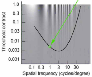
 This method has an experimenter (or computer) decrease (continuously or stepwise) the magnitude of a physical property of a stimulus until the participant reports that it has just disappeared. That is alternated with increasing that magnitude until the stimulus first appears. (It just makes sense to go back and forth a bit when selecting a setting precisely.) The threshold is obtained by averaging the levels at which the stimulus disappears with the levels at which it first appears. Here is a hypothetical example of measuring the contrast sensitivity thresholds of spatial frequency patterns from 0.1 to 40 cycles per degree.
These measurements were obtained with a 1.0 cycle per degree (cpd) grating, initially presented at a 0.02 light-to-dark contrast setting, at which the light and dark bars were visible. The experimenter stepwise or continuously reduced the contrast until at 0.0054 contrast, the participant signaled that the bars disappeared. The experimenter then reduced the contrast further and then slowly increased it. The participant signaled that the bars became visible at 0.0076.
The table below shows eight such measurements. The mean of these readings equals the threshold contrast for that spatial frequency. These measurements would be repeated for 0.1 to 40 cpd spatial frequency patterns to complete the function shown in the figure.

1.2 Method of Adjustment
This method is similar to the Method of Limits, except that the participant increases and decreases the stimulus magnitude. The measurements and their analyses proceed in the same manner. With experienced participants, the Method of Adjustment is more efficient, sensitive, and engaging for the participant, though possibly less objective than the Method of Limits.
1.3 Methods of Constant Stimuli
The Method of Limits and the Method of Adjustment are weakened by the participant’s tendency to anticipate whether the next stimulus is likely to be visible or not. This is avoided by presenting the stimulus levels in pseudo-random order, ensuring each level is presented an equal number of times. This objectivity is gained at the cost of complicating the threshold calculation, as shown in this example:
The time course of how visual thresholds decrease in darkness is difficult to measure due to the initial rapid decrease in the amount of light that can be detected. Yet, this method works well.
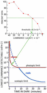
The participant is comfortably seated with a headrest to hold eye position steady. A dark screen displays a set of dim crosshairs to direct the participant’s gaze. After 5 minutes to fully adapt to a room illumination set to 100 lumens/meter2 (outdoor lighting on dark day – see endnote 101), the lighting is turned off, and a timer started. At 5 seconds, a beep indicates the onset of a ½ second spot set to a specific brightness. The participant presses a button if the spot is seen. Twenty seconds later, this is repeated with the spot set to a different brightness. This procedure continues for 30 minutes. Then the room lighting is turned on, and the participant rests for a few minutes.
This procedure is repeated with different levels of spot brightness at 20-second intervals. After 2-3 hours, the testing would end for that day and resume on following days. To measure the detection of eight different levels of spot brightness at each interval would take 240 of these 35-minute sessions to obtain 30 measurements of each brightness level. Given an expected change in sensitivity by a factor of 105, extensive preliminary testing is required to select only eight spot brightness levels to test at each 20-second interval without biasing the results. (Too wide a range of test levels would not provide accurate measurements at that duration, and risk losing the participant’s attention if many levels were either obvious or not seen.)
For each 20-second test interval, the number of seen spots is plotted with respect to spot brightness. The brightness at which 50% of the spots were seen defines the threshold at that interval after the room became dark. These analyses are repeated for each of the 150 20-second intervals to show how sensitivity to light increases over 30 minutes after darkness begins.
However, this simple procedure is rarely used due to a potential problem. There is no way to tell if the participant may be too “helpful” and think they see something at every level, or too “demanding” and find even the strongest level doubtful. A modest procedural change can avoid this.
2-Position Forced-Choice
Present two spots side-by-side every time, with one (selected randomly) containing the test luminance and the other blank. The participant reports which spot had some brightness. These measurements are analyzed the same way in terms of “percent correct”, but with 75% correct defining the threshold. (Just guessing would be correct half the time.) It also makes the task easier for the participant. Even for persons experienced in making these measurements, it is not easy to hold a consistent idea of a dim brightness while sitting in darkness. A further procedural variation removes almost all conceivable subjectivity.
3-Position Forced-Choice
Present three spots each time, with only one containing the test luminance and the other two being blank. The participant now indicates which one was different. 66% correct now defines the threshold, since the correct choice can happen by chance one-third of the time. This version of the Method of Constant Stimuli is more sensitive and objective than the other methods of measuring thresholds. It is also the most time-consuming and often requires complex apparatus. Because these factors make it the most expensive psychophysical method, it is not often used – especially when research funds are tight, and there is pressure to publish.
2. Difference-Threshold Measurements
Thresholds only describe the operation of a system at its lowest limit. Yet systems rarely operate at that level. Difference-thresholds show how systems operate at normal levels. They can also provide more insight into underlying processes than thresholds.
For example, compare: the thresholds for seeing color with color difference-thresholds.
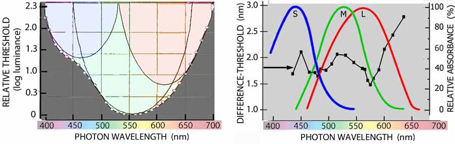
Irregularity in the threshold function hints at 2 or possibly 3 underlying processes. Calculus applied to the difference-threshold function reveals 3 functions that approximate the absorption characteristics of the three types of cone photoreceptors. Unfortunately, this additional knowledge is costly: 1) many more measurements are needed; 2) the required equipment is often more complex.
2.1 Method of Limits & Method of Adjustment
The simplest versions of these methods asks the participant to signal when the appearance of a stimulus has changed as a result of some physical property, such as its luminance, orientation, or wavelength, is changed. For a specific level of that property, the level is gradually increased or decreased until the participant signals that the stimulus has changed. Tests with the level being increased alternate with tests that decrease it. The analysis is the same whether the experimenter or the participant makes the changes, and whether the changes are continuous or step-wise. The increments and decrements are averaged separately. Half their difference defines the difference-threshold for that specific level. These measurements are then repeated at more levels to cover the range of that stimulus property.
2.2 Method of Constant Stimuli
The simplest version of this method presents two stimuli: one at the specific physical level being measured, the other set to a particular physical difference from that level. The participant reports whether they looked the “same” or “different”. Various magnitudes of difference are tested repeatedly in a pseudo-random order. The smallest difference that is detected 50% of the time provides the difference-threshold. Unfortunately, this simple approach leaves the participant’s effort or basis of the decision unknown.
A “2-Position Forced-Choice” version is less dependent on the participant’s subjectivity. The participant reports which randomized position had the larger magnitude of a specific quality, such as brightness, size, or beauty 75% correct now defines the difference-threshold. This controls what particular quality difference is being measured, and provides a check on the participant’s effort.
The “3-Position Forced-Choice” version makes one of three stimuli different in magnitude. Its position is randomized. The level that is correctly selected as different 66% of the time defines the difference-threshold. As with its use to measure thresholds, this is the most objective, sensitive, and costly way to measure difference-thresholds.
3. Stimulus Matching Methods
Chapter 13 described how Benjamin Thompson’s use of equal brightness judgments to measure light was a forerunner to using physics to measure brightness and scientifically studying the mind. In adjusting the distances of the lamps to obtain a match, he was using the visual system as a null instrument – a most sensitive and precise measurement method used in science and engineering. It bypasses nonlinearities and biases in the measuring instrument, be it a physical device or a human. This makes it comparable in sensitivity and objectiveness to the 3-Position-Forced-Choice. Like the methods that have the participant adjust the test stimulus, measurements obtained by matching are efficient and interesting for the participant.
3.1 Measuring Difference-Thresholds
This method of measuring difference-thresholds differs from the other methods by asking the participant to report when two stimuli are the same. How can that measure the ability to see a difference? Bear with me.
For example, here is how to measure the accuracy of our ability to see the angle of a line at various angles. Present two lines of the same size and brightness. One line is set at the angle whose difference- threshold is being measured. The angle of the other is adjusted to match former. The adjusting can be done either by the experimenter or the participant. The initial angle of the adjustable line is alternated between being greater or smaller than the angle being tested. When enough pairs of matches have been made, they are averaged. Not surprisingly, their mean will be close to the angle being measured. However, that is of little interest. What is of interest is that the matches vary more for angles that have a larger difference-threshold. The standard deviation of the matches defines the difference-threshold.
(See Appendix I – A Little Statistics). The table shows results for matches to a 65o angle:
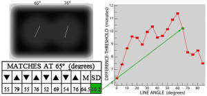 These matches would be repeated with the left line set to each of the other angles from 0o to 85o to obtain the function shown in the figure.
3.2 Cross-Modality Matching
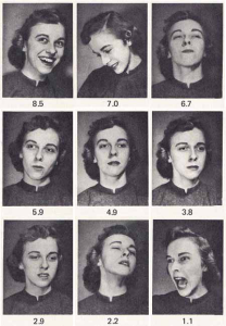
From art auctions to safety signs, innumerable images call for measurement and comparison of their effectiveness, but their physical properties are too complex for direct measurement. Various methods are used to cognitively relate some attribute of such images to something that can be directly measured. For example, measurements of the strength of facial emotions by matching pictures of faces to numbers have proven useful in a range of clinical and social applications, such as diagnosing pain and evaluating quality of life.
Engen, Schlosberg & Levy (1958) provide an example of measuring facial emotions. They had 96 students use a 9-point scale to rate a series of facial photos that expressed various degrees of specific emotions.[1] This figure shows the medians (averages) of their pleasantness ratings of a person whose expressions varied from pleasant to unpleasant:
Cross-modality matching was the best way to match stimuli of different wavelengths in terms of the visual effect of brightness despite their color differences. Shown in Ch 14, the results are the basis of photometry.
4. Reaction Time Measurements
The basic method has a participant prepared to look for a specific stimulus such as a shape, color, or symbol. The participant is instructed to release a key the moment they see that stimulus. A clock is started when the stimulus is presented. The clock stops when the key is released. The method’s simplicity soon led to measuring reaction times to all sorts of stimuli, with many additional variables, such as the participant’s condition, task difficulty, and test environment. An example of early attempts to relate psycho-physical measurements to visual neurophysiology is A.T. Poffenberger’s (1912) measurement of reaction time to stimuli presented to different locations on the retina is. His results resemble the distribution of retinal rods and cones (see fig. in Ch 24). This led him to attribute the reaction time differences to the number of synaptic delays involved in the processing. [2]
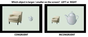
One hundred years later, Tala Konkle & Aude Oliva (2012) used reaction time to study the visual system’s processing to compare retinal image size with perceived size. [3] Participants were asked to quickly indicate which object was the larger (or smaller) image. When those images were incongruent with the object’s real size, participants took 50 milliseconds longer to decide than when the retinal image sizes were congruent with their real size. As Poffenberger might put it, “At a 0.5 millisecond delay per synapse, that’s a lot of additional synapses.”
- Engen T, Levy N & Schlosberg H (1958) The dimensional analysis of a new series of facial expression. Journal of Experimental Psychology, 55, ↵
- Poffenberger AT, Jr. (1912) Reaction time to retinal stimulation. Archives of Psychology, No. 23. ↵
- Konkle T & Oliva A (2012) A familiar-size Stroop effect: Real-world size is an autonomous property of object representation. Journal of Experimental Psychology: Human Perception and Performance, 38, 561-569. ↵