
APPENDIX I – A Little Statistics
As matters get complicated, understanding what is happening is often not evident at first sight. (That’s why they seem complicated.) It can require many observations before we know what is happening. Yet, in the real world, more measurements are never quite the same – no matter how carefully one measures. But then, working with a bunch of measurements becomes impractical. The solution is to summarize a bunch of numbers by averaging them. The following illustrates how some simple statistics have proven to be essential in brain research.
A basic approach to learning how something (including a brain) works is to do something to it and see what happens. However, complicated things constantly tend to change somewhat. Since the combined effects of many variables can appear random, focusing on a particular variable may benefit by treating the effects of the others as random. Fortunately, even randomness obeys specific laws regarding variability. These enable statistics to determine whether measurements made before and after doing something showed an effect that was unlikely to be random despite their variability.
Sometimes it is important to learn if one set of measurements is similar to another set. For example, is there a similarity in the brain`s responses to two stimuli? Are similar responses in two areas of the brain an indication of being linked? Determining whether a similarity of two sets of complex measurements is real or due to chance may seem a task for artificial intelligence. Still, a relatively simple statistical calculation, correlation can do this.
AVERAGES
Most readers know how to find what is commonly called an “average”: You add a set of numbers and divide the sum by how many numbers were added. That average is more specifically called a mean. In this book, that is what the term “average” usually means.[1] Besides providing the best unbiased description of a bunch of measurements, means are also a powerful yet simple way to reduce random effects in measurements. This makes them especially valuable for studying the brain’s activity.
A lot happens in complex systems, like the brain, that is not relevant to a specific effect of interest. Many other effects can completely obscure that specific effect. However, if the other effects occur independently of that particular effect, they can be largely removed by averaging.
To use electroencephalography (EEG) to see the brain’s response to a specific image:
 1. Present the image for a 1/2 second.
2. Simultaneously start recording the EEG for up to 1 second.
3. Pause for several seconds.
4. Repeat the above steps 60 times.
5. Average the records.
Each time the image is presented, the activity in the rest of the brain differs. When added together, the records of those other activities tend to cancel each other, leaving just the sum of the response to the repeated image.
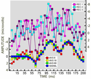
Here are 250 ms records of a repeated signal mixed with a random signal:
The upper three single records ( ■, ■, ■ ) bear little resemblance to the actual signal shown below in blue.
An average of just 6 records shows some similarity to the blue signal. The average of 60 records is very similar to the actual signal. [2]
STANDARD DEVIATIONS
As illustrated above, single EEG measurements of the brain’s response to an image look random when repeated. Despite all the other effects contributing randomly to those repeated measurements, you may be surprised to learn that their combined effect is not random!
A simple example of a random effect is the outcome of a flipped coin. Though each outcome is random, half the time the coin comes up Heads – in the long run. Now flip 6 coins, and count the number of Heads. You soon realize that the total number of Heads usually differs each time, and that there are 7 different totals ranging from all Heads to all Tails. Moreover, some totals occur more frequently than others – even in the long run. “How is that possible when each coin comes up Heads half the time?”
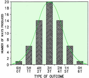
You knew the answer, but may not have fully considered its implications: You can only get 6 Heads when every coin comes up Heads, but there are many different ways that half of them can be Heads. (Without resorting to Probability Theory, six coins can demonstrate the 20 ways.) It only makes sense that outcomes that can happen in more ways happen more often. There are 64 possible outcomes from flipping six coins. They are split up like this:
It is called a normal distribution because random events usually spread out this way. If Heads were valued “1″ and Tails “0″, the result of averaging 64 flips would be close to “3″ most of the time.
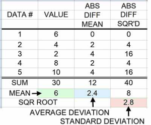 While averages can reveal a consistent response in a complex system, repeating the measurements usually results in a different averages. There is a way to tell the reliability of an average based on the variability of its measurements. Basically, how big is the average compared to the extent of that variability?
The variability of a set of numbers is also describable by averaging: how much each number differs from the set’s mean value – their average deviation (AD) from that mean.
That set’s variability can also be calculated with another average that is unfamiliar to most people: a “root-mean-square average” (square each difference; sum the squares; divide by the number of squares; take the square root of the dividend): The latter average is also called a standard deviation or SD because it is the measure of variability that is generally used.
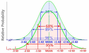
Both variability descriptions are systematically related to normal distributions: 58% of all values tend to be plus and minus 1 AD from the mean value, and 68% of them within plus and minus 1 SD from that mean.
However, you don’t have to take that for granted:
Flipping more coins more accurately simulates most random effects, resulting in a closer approximation to a normal distribution. Here are the results from flipping 20 coins:
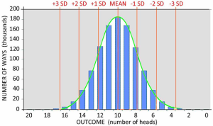 The 1,048,576 possible out- comes result in a smoother distribution and a closer approximation to having 68% of the outcomes within plus and minus one SD of the mean outcome. (I came close, but on the last flip, I got a second set of all heads.) Ideally, this is their distribution:
Most factors encountered in averaging cortical responses are neither binary nor normally distributed in their effects. They tend to be random only with respect to the specific effect being measured. Just as each coin is not normally distributed in its outcomes, when many coins or cortical responses are combined their averages are normally distributed.
A little patience, counting, and simple arithmetic are all you need to further demonstrate a basic principle of the universe as fundamental as E = ½ Mc2:
Roll four die hundred times. Find the mean and the standard deviation (SD) of the outcomes. See if 68% of the outcomes are within plus and minus 1 SD of the mean. A spreadsheet makes this easy. Copy 100 of RANDBETWEEN(1,6) into four columns. Sum each row and Convert to Values the sums in a new column. Arrange those values in ascending order. Calculate their mean and standard deviation. Then count.
This universal property of randomness forms the basis of statistical tests to determine whether two or more means are different. A difference between two means that is greater than twice their joint standard deviation is less than 5 percent likely to be a random difference. By convention, their difference is then considered to be significant.
For example, in the lower figure chapter 29 under Binocular Disparity, these evoked potentials were measured every 2.5 ms from the moment a stimulus was presented until 500 ms later. Various independent cortical effects contributed to the voltage recorded at each interval. Repeating these measurements 90 times cancelled out the non-related effects. Though how each of hose effects varied over time was unknown, the distribution of some of their averages would be normal. This enabled comparing the means of the certain and uncertain sets of responses measured at each 2.5 ms interval based on the variability of the mean voltage at each interval.
Tests like these are based on SDs and not ADs. Why? The larger root mean square average of differences from a mean more accurately represents the information uncertainty of each number than the average of each number’s difference from the mean. Why? The reason involves another universal property – the connection between energy, information and the 2nd Law of Thermodynamics. Therein also lies the explanation of why higher temperature and voltage values do more work than suggested by their difference from lower values, e.g., diesel versus gasoline engines; 220 VAC industrial motors versus 120 VAC hobby drills. We’ll skip the theory with the following demonstration.
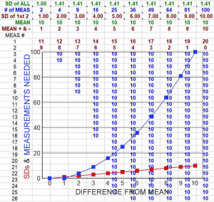
Shown are ten sets of measurements, all with a MEAN 10 . From left to right, the first two measurements differ from the mean by plus and minus 1, 2, 3, …to 10 in the last column. The row above the MEANs shows the SDs of the 1st TWO measurements. As expected, these SD’s increase linearly with the first measurements’ differences from the mean. However, the increase in uncertainty about the mean caused by those differences is not linear. That uncertainty is indicated by how much work is required to reduce the uncertainty to the 1.41 SD of ALL four measurements when the first two measurements differed from their mean by “2“. The minimal “work” would involve further measurements that equaled the MEAN.
To obtain the same low value of uncertainty, the number of such added MEASUREMENTS NEEDED increases with the square of the difference from the mean:
CORRELATIONS
Comparing the complex activity recorded from different areas of the brain or recorded at different times does not require artificial intelligence to tell if they may be related. In 1888, Francis Galton found a way to describe the similarity of two sets of numbers; but Karl Pearson’s 1894 invention of the standard deviation was needed to make the method practical. Unfortunately, correlations are often misunderstood. That is partly due to statistics books using complicated formulas for calculation and explaining their use for linear equations. Though a bit tedious, the simplified method below may help –if you understand standard deviations. See above.)

To objectively specify the similarity of these two sets of numbers:
1. Put them on a common level by subtracting a set`s average from each number in that set: This converts them into relative values.
2. Make their variability proportional to the set’s average. Divide each relative value by the standard deviation of that set`s relative values: This produces the two sets of “Z” scores.
3. Multiply the pairs of Z scores together. When corresponding Z scores in each set are positive (above average), or both are negative, their product is positive: This indicates a similar trend as both values were either above or below their set’s average value at that moment.
When one Z score is positive and the other is negative, their product is negative: This indicates the two sets had opposite trends at that moment.
4. The average of these Z products indicates the overall degree of similarity – i.e., the correlation. Correlations are typically denoted by the symbol “r”. Tables from the web and introductory statistics books list the value of the Pearson Correlation Coefficient, “r”, that is required for a correlation to be only 5% likely due to chance. The “size” required for a correlation to be significant decreases with more pairs of numbers.
A graph of the above two sets of numbers suggests some tendency for both sets’ values to increase with time:
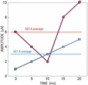
However, this trend is not statistically significant. Five numbers in each set are too few for a correlation of either 0.6 or -0.6 to be significant. A Pearson Table shows that 5 pairs of numbers require a correlation of 0.73 to be confident that this similarity (or dissimilarity) could happen by chance, only 5% of the time.
Bear in mind that negative correlations also indicate a relationship. Learning that two sets of measurements show opposite effects can be as valuable as learning that they are similar.
On the other hand, correlations near zero suggest That the two patterns of activity may be independent. This can also be worth knowing.
A caveat applies here: Correlations only indicate the strength of a linear relationship between two sets of measurements. Consequently, correlating measurements such as visual acuity and spatial frequency would suggest that they are poorly related! That’s because acuity increases at low frequencies, then decreases at frequencies above 3 cycles per degree. See Ch 27.
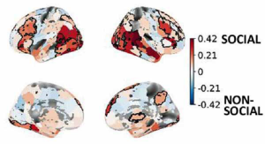
In the following example, correlation calculations enabled locating cortical areas that selectively respond to a complex yet subtle aspect of visual images – whether they show social interaction. Recha Varrier & Emilj Finn had participants view 20 sec movie clips that showed persons in either social or non-social scenes. [3] Correlational analysis of the fMRI responses identified numerous areas that were selectively sensitive to social interactions.
Comparing patterns of activity in different brain areas is complicated by the neural conduction times. For example, the ear is closer to the auditory cortex in the temporal lobe than the eye is to the visual cortex in the occipital lobe. (See Appendix E.) Therefore, the auditory response to an event reaches the auditory cortex about 20 milliseconds sooner than the visual response reaches the visual cortex. Similar conduction delays complicate the use of correlations to compare responses in different regions of the cortex. Cross-correlations provide a simple, though tedious, solution. Calculate the correlations repeatedly while shifting one response stepwise with respect to the other. A sudden increase in r at a particular step indicates a similarity despite the relative difference in time of occurrence.
There is a further lesson to be gained from cross-correlation calculations. What they do and the equation for each calculation looks complicated:

However, the above table reveals that the actual calculation is just a lot of simple steps in arithmetic.
X are the values of one set of measurements
Y are the values of a second set
n is the number of measurements in each set
These statistical calculations show that complicated processing can be the result of many simple processes. After all, is that not how the brain works: thousands and millions of neurons, each producing a small effect, yet somehow these effects merge? Appendix I showed that a signal could be extracted from noise with a small number of averages. Population encoding can effectively portray a large number of details with relatively few channels. On such bases that may not require as many nor as complicated operations as you might think. From that perspective, we may eventually understand how the picture-in-your-head happens.
- Other `averages` include the median, which the middle value when a set of numbers is arranged in ascending order; the mode which is the value of that occurs most often in a set; and the root mean square (rms), which is of special significance in physics when describing the ability of a varying voltage or temperature to do work. That is why audio amplifiers are rated in terms of rms watts. So the uncertainty about a mean caused by varying differences from the mean of a set of measurements is proportional to the rms average of the differences. ↵
- Sutton, et al, 148, averaged 90 EEGs. Had those results not been consistent, they would have dumped their CAT 200 averager.) ↵
- Varrier RS & Finn ES (2022) Seeing Social: A Neural signature for conscious perception of social interactions. The Journal of Neuroscience, 42, 9211-9226 {https://doi.org/10.1523/JNEUROSCI.0859-22.2022}. ↵