
IV. STEPS TOWARDS CONSCIOUSNESS
30. LOOKING INTO THE BRAIN
Electrodes
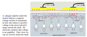
Information about the brightness, color, size, and location of even a brief flash is conveyed by hundreds of nerve fibers sending thousands of 40mV action potentials. While each only lasts a millisecond, their effect on the fluid outside the neurons adds up. Fortunately, most of the visual (as well as auditory and touch) information is processed in that 3 mm thick sheet of neural tissue directly under the skull.
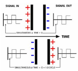
Like two magnets of opposite field following each other although separated by a tablecloth, capacitive coupling enables following cortical electrical changes from outside the skull: An accumulation of negative ions inside a membrane repels electrons on the outside, inducing a positive charge. Positive ions inside a membrane attract electrons on the outside, inducing a negative charge.
 Amplifiers
Dissipated by passing through the dura tissue enclosing the brain, the skull, and the covering skin, the voltages that reach outside the skull are weak – in the microvolt range, compared to nerve impulses. Tracking these weak signals requires substantial amplification. A simple principle describes how most amplifiers work.
But first you should know: Most amplifiers do not amplify signals!
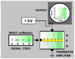 Instead, they use a weak signal to control a stronger steady voltage.
This transistor amplifier consists of a semiconducting P layer between two N layers that only conducts electrons in one direction (up). The P layer is non conductive until a weak voltage is applied.
The transistor conducts more electrons as the applied voltage increases. If the applied voltage is a signal that varies with time, the amplifier’s output will vary the same way, so it looks like the signal was amplified. Amplifiers just copy a signal as it changes.
Above, a 3 millivolt input results in 3 volts from the power supply flowing through the transistor. The millivolt signal is “amplified” by a gain of 1000X.
Seeing the Brain’s Electrical Activity
In 1920, weak fluctuations of a galvanometer probe during brain surgery led Hans Berger at the University of Jena to the brain’s electrical activity. He connected a vacuum tube amplifier to the galvanometer and found he could record this activity from outside the head with electrodes on the scalp. These “electroencephalogram” (EEG) waves had different frequencies depending on the participant’s behavior and named them:
Gamma > 60 Hz movement and cognitive efforts
Beta16 – 40 Hz active thought, movement, dreaming
Alpha8 -14 Hzawake but resting (discovered first)
Theta 4 – 8 Hzdeep sleep
Delta< 3 Hzcomatose
Brain activity related to specific operations such as inhaling, moving a hand, hearing a bell, remembering breakfast, etc., is superimposed on these rhythms.
The capacitive coupling that extends the neural electrical field outside the head is problematic. It is only partly local to the cortex directly below the electrode. Furthermore, much of the brain’s activity involves unconscious operations, such as control of bodily functions. Therefore, when seeking to record the brain’s response to a specific visual stimulus, that response also contains the combined electrical fields of all the other brain activities to varying degrees. An electrode placed over the occipital lobe picks up not only the visual response but also the electrical fields radiating from throughout the brain. Consequently, when trying to see the visual system’s response to a specific stimulus, the obtained EEG response differs every time that stimulus is presented.
Averaging EEG signals, and then correlating their average with what was shown is a widely used tool to determine how brain responses relate to a picture-in-the-head. Though simple calculations, they are often misunderstood. To see how they work for studying the brain, go to Appendix I – A Little Statistics. The results of EEG signal averaging are called cortical evoked potentials.
Prior to the availability of computers, students were employed for hours after each experiment to tabulate and average EEG voltage tracings with calculators. In the early 1960s, studies of the electrical activity of the human brain were revolutionized by using computers to do the averaging.
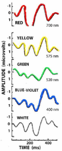
Here are the cortical evoked potential results of two studies that used early computers to look at how the human brain responded to different colors and how the brain responded differently depending on a cognitive factor – the novelty of the stimuli. [1]
These records were consistent and distinctive enough to tell the researchers what color the participant had seen:
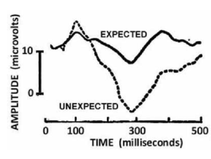
Here is the first evidence of a cortical response related to a cognitive aspect of a visual stimulus. Note the stronger response when the stimulus was not expected. This occurs about 300 ms after the stimuli are presented.
Recording from many locations over the head enables estimating where a specific evoked potential pattern originated – despite the overlapping electric fields.
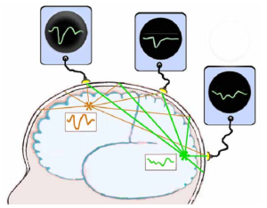 Here is a simple example of how that works:
This person looked at something green but happened to think about red at the same time. Characteristic evoked potential patterns for ‘green’ and ‘red’ were recorded over the occipital and frontal lobes. Halfway between these electrodes, an electrode over the parietal lobe records a weakened pattern that is half red and half green. It will be more similar to the parietal cortex activity than the frontal cortex.
Computer analysis compares the similarity of activity in the occipital cortex with activity in other locations by calculating their correlation.
The most likely location for each pattern is extracted by comparing the pattern from every electrode with the patterns from surrounding electrodes. (These locations may not be exactly where the electrodes are placed.
Based on the locations of the recording electrodes, trigonometry enables mapping these responses with respect to the brain’s anatomy. This is the basis of the tomographic displays that are also used with acoustic reflections, and x-rays to construct 2- and 3-dimensional pictures of structures in the brain and body.
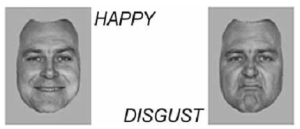
Utama, et al (2009) found that cortical evoked potentials can distinguish visual responses to faces expressing:
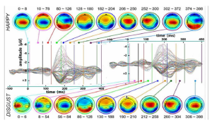 At about 200 ms after the faces were shown, peak responses to the happiness faces occurred about 10 milliseconds sooner than the peak response to the disgust faces. [2]
The above evoked responses were recorded from different electrode locations on the scalp. Applying trigonometry to the signals from these locations enabled mapping their amplitude differences across the brain. Because the ions carrying these electric potentials diffuse while passing through the neural tissue, skull, and scalp, more precise location of where these responses occurred is not possible.
An alternative approach to looking inside the head proved to have the opposite characteristics: excellent determination of the location of neural activity but poor measurement of when it occurred:
Magnetic Resonance Imaging
In 1937, Israel Rabi at Columbia University discovered a delicate effect that an oscillating magnetic field had on lithium chloride molecules lined up peacefully inside an enormously strong, 0.2 Tesla magnetic field. (That equals about 2 million fridge magnets.) When exposed to a resonant 3.5 MHZ electromagnetic (e-m) probe from another direction, the LiCl molecules reorient in that direction as they absorb this energy. When this e-m field is turned off, the molecules return to their peaceful orientation and release 3.5 MHZ radiation.
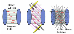
Though this obscure effect was only detectable under precise conditions, it earned a Noble Prize in 1944. Why? Further study by physicists and chemists led to:
1. new insights into the quantal nature of atomic nuclei,
2. non-optical spectroscopy to identify unknown substances,
3. A new means of determining the structure of complex molecules, and 4. magnetic resonance imaging (MRI) – a more precise, benign, though expensive alternative to x-ray diagnostics.
Mapping Brain Structure
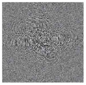
In 1973 Paul Lauterbur at New York State Stoneybrook University introduced a means of converting MRI signals into images. He applied Fourier synthesis to the diffraction patterns produced by the photons radiating from the locations of the emitting molecules:
Tuned to the resonant frequency of water, MRI could distinguish the density of various human body tissues in terms of signal strength relaxation times.
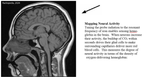
M
These figures show a series of fMRI scans sensing the neural activity in length-wise, cross-wise, and horizontal planar sections of the brain when persons saw motion, looked in specific locations, viewed whole bodies (minus head), and viewed body parts. [3]
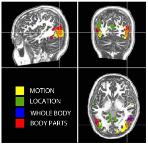
Note the more localization of these different responses compared to the EEG based evoked potentials in the figure in Ch 30. However, exactly when the fMRI responses occurred can not be determined. It takes a few seconds to induce and then release the effect.
(Stronger electromagnets and more sensitive e-m amplifiers can improve the temporal and spatial resolution. However, strong electromagnets draw large currents that require cryogenic cooling to obtain super-conductivity and prevent the magnets from melting. The costs limit their use in vision experiments.)
Diffusion Tensor fMRI
Rapid operation of sodium-potassium pumps during the refractory aftermath of a nerve impulse (Ch 11) is accompanied by water molecules cycling through the neural membrane. As the impulses spread along the nerve fiber, these water molecules diffuse along the nerve bundles connecting different brain areas. By orienting the magnetic fields and the electromagnetic probe and pulsing the probe, it is possible to sense the movement of these cycling water molecules in selected directions.
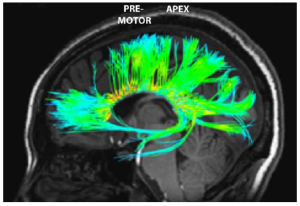
Asking a person to attend to specific visual stimuli during this procedure shows where those neural responses go in the brain. This figure shows neural tracts connecting the occipital, frontal lobes and parietal lobe during a visual task. [4]
This measurement is almost as fast as the EEG response. However, this measurement is sensitive to the slightest head movement. This makes it expensive and difficult to incorporate in experiments.
Transcortical Magnetic Stimulation (TMS)
Placing some battery-powered tools on an alternating current (AC) electromagnet induces a current in an inside coil and charges them. Similarly, a powerful magnet placed on the head can capacitively induce, through the skull, an ionic current in underlying nerve fibers. Since the induced ion flow is unorganized, the usual result is disruptive. In that manner, TMS can temporarily block neural signals without adverse side effects.
Due to the distance from the electromagnet to the neurons and the fact that only some axons or dendrites will be favorably aligned for induction, a powerful 2.5 Tesla magnetic field is required. This can be obtained with an 8,000 Ampere pulse for about 1/10th of a millisecond (ms) without melting the magnetizing coil. The resulting electric field can be localized to a few centimeters.
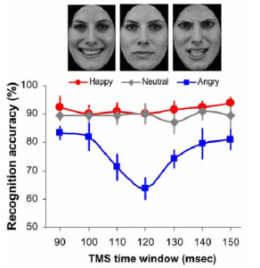
Guo, et al applied a single TMS pulse above the left visual cortex at 90 to 150 milliseconds after a brief presentation of a face having either a happy, neutral or angry expression. Participants reported which emotion was shown. [5]
TMS pulses applied 120 ms after the faces were shown substantially decreased accuracy of recognizing angry faces but did not reduce the accuracy of recognizing either the happy, or neutral faces at any time.
This suggests that recognition of anger, but not happiness, gets added about 120 ms after the faces are seen. (TMS probes at other locations might reveal the origin of that emotional input.)
Other Methods of Measuring Brain Activity
There are many more methods of measuring what is happening in the brain during vision, and more are discovered every year. Near-infrared optical topography is another non-invasive method, though less used than those above: It directs an intense beam of infrared light through the scalp and skull. The amount of reflected light is proportional to the density of red blood cells, which gather to provide oxygen where the cortex is most active. It is less expensive than fMRI, can localize responses to about a centimeter, but it is limited to outer cortical surfaces. It does not require applying electrode paste to the scalp as does EEG recording. It works particularly well with infants due to their thinner skulls. [6]
Most other methods are invasive techniques and generally unsuitable, even for use on graduate students. These methods include: a) inserting needles into the brain to record and electrically stimulate; b) using pipettes to inject chemicals such as neurotransmitters, or to sample chemicals; c) inserting optical fibers to stimulate injected photoreactive compounds, or to record responses from injected fluorescent dyes; d) genetic altering of structures and sources of neuroactive chemicals by injecting genome editing bacteria. They apply only to animal research, except for special clinical situations with humans when surgery is happening for other reasons.
Animals can be taught to indicate when they have seen a specific visual image by rewarding them with treats or punishing them with mild shocks. For example, by pressing a lever when, and only when, a pattern of lines has tilted, or by moving towards the light of a specific wavelength, or by touching the projected image that is different from two other images. Whether simpler animals such as sea slugs experience a visual image or behave reflexively is unknown. Nevertheless, experiments with their behavior and neural responses can reveal how basic mechanisms process visual information.
For more information about the above and other methods, see Carter M, Essner R, Goldstein N & Iyler M (2022) Guide to Research Techniques in Neuroscience, 3rd Edition, ISBN 978-0-12-818646-6, Academic Press.
- p. 148 Shipley T, Jones RW & Fry A (1965) Evoked visual potentials and human color vision. Science, 150, 1162-1164. Sutton S, Braren M, Zubin J & John ER (1965) Evoked potential correlates of stimulus uncertainty. Science, 150, 1187-1188. ↵
- Utama, NP, Takemoto A, Koike Y & Nakamura K (2009) Phased processing of facial emotion: An ERP study. Neuroscience Research, 54, 30-40. Figure 4 used with permission. ↵
- Figure modified from Downing PE, Wiggett AJ & Peelen MV (2007) Functional magnetic resonance imaging investigation of overlapping lateral occipitotemporal activations using multi-voxel pattern analysis. The Journal of Neuroscience, 27, 226-233, Fig. 2 {doi:10.1523/JNEUROSCI.3619-06.2007}. ↵
- Diffusion tensor fMRI image used by permission from Lawrence Frank, Ph.D., Director, Center for Scientific Computing in Imaging (csci.ucsd.edu). ↵
- Figure modified from Guo K, Calver L, Soornack Y & Bourke P. (2020) Valence-dependent disruption in processing facial expressions of emotion in early visual cortex - A transcranial magneticstimulation study. Journal of Cognitive Neuroscience, 32, 906-916, Figs. 1 & 4 {doi.org/10.1162/jocn_a_01520}. ↵
- Collins-Jones, et al (2024) Whole-head high diffuse optical tomography to map infant audio-visual responses to social and non-social stimuli. Imaging Neuroscience, 2 {https://doi.org/10.1162/imag_a_00244}.Higher intensity light sources and more sensitive detectors may extend photon brain scanning to adults and enable mapping brain activity as well as structure - Radford J, et al (2025) Photon transport through the entire adult human head. Neurophotonics, 12, 2, 025014 {https://doi.org/10.1117/1.NPh.12.2.025014}. ↵