
Chapter 6: Internal Forces
6.2 Shear/Moment Diagrams
6.2.1 What are Shear/Moment Diagrams?
Shear/Moment diagrams are graphical representations of the internal shear force and bending moment along the whole beam.
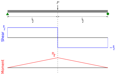
Shearing Force Diagram
This is a graphical representation of the variation of the shearing force on a portion or the entire length of a beam or frame. As a convention, the shearing force diagram can be drawn above or below the x-centroidal axis of the structure, but it must be indicated if it is a positive or negative shear force.
Bending Moment Diagram
This is a graphical representation of the variation of the bending moment on a segment or the entire length of a beam or frame. As a convention, the positive bending moments are drawn above the x-centroidal axis of the structure, while the negative bending moments are drawn below the axis.
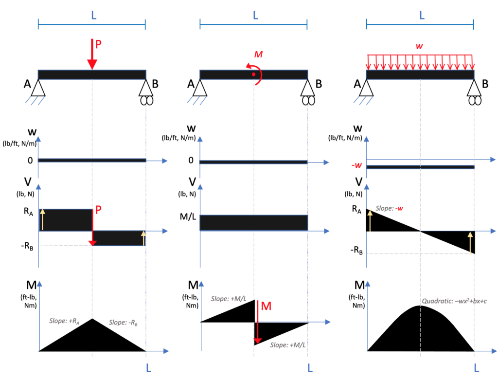
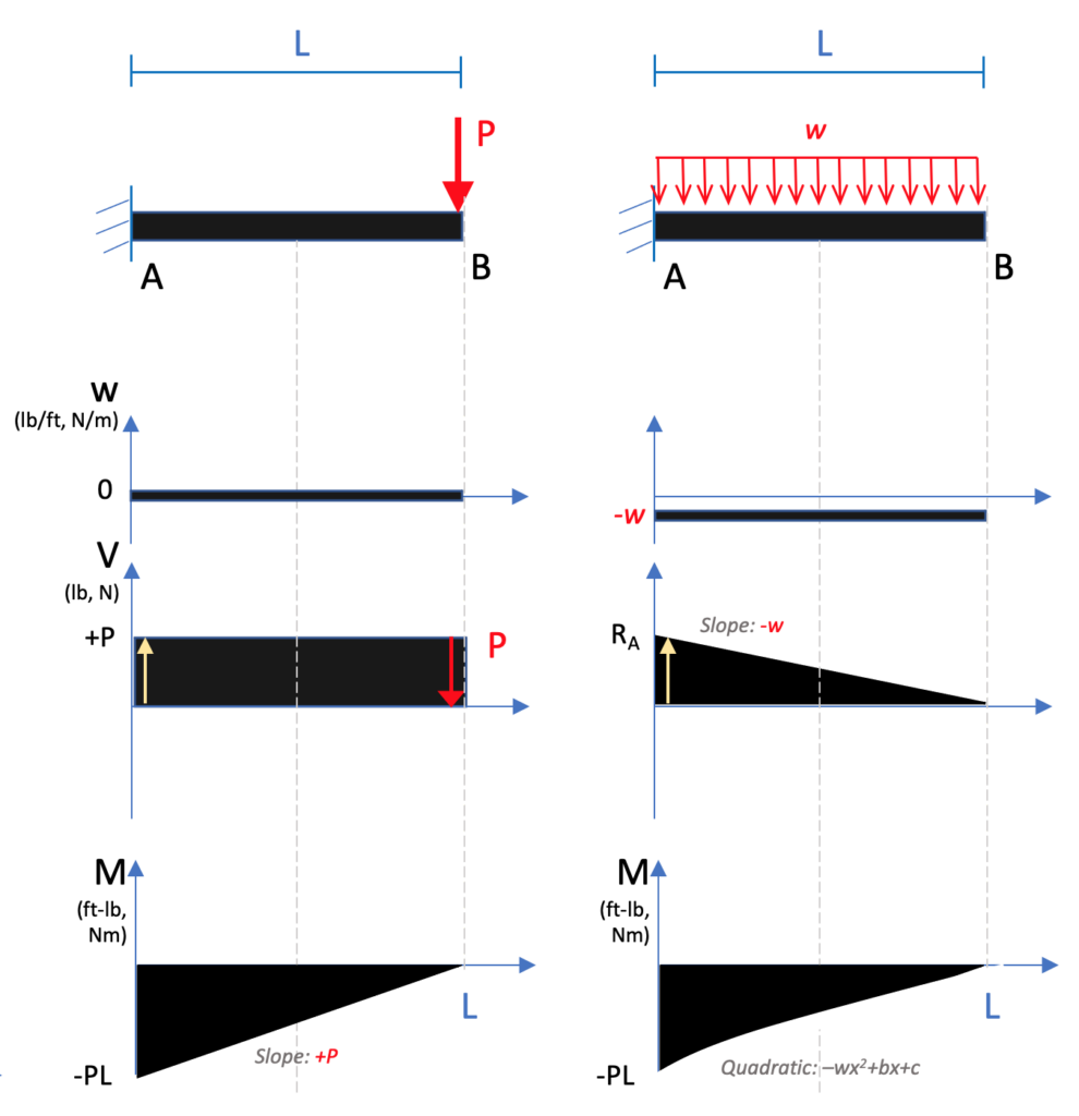
Below is a simple example of what shear and moment diagrams look like. Afterwards, the relation between the load on the beam and the diagrams will be discussed.
Source: Internal Forces in Beams and Frames, LibreTexts. https://eng.libretexts.org/Bookshelves/Civil_Engineering/Book%3A_Structural_Analysis_(Udoeyo)/01%3A_Chapters/1.04%3A_Internal_Forces_in_Beams_and_Frames
6.2.2 Distributed Loads & Shear/Moment Diagrams
There is a relationship between distributed loads and shear/moment diagrams. Simply put:
[latex]\frac{dM}{dx}=V(x)[/latex]
[latex]\frac{dV}{dx}=-w(x)[/latex]
[latex]\frac{d^2M}{dx^2}=-w(x)[/latex]
Or:
[latex]\Delta M=\int V(x)dx[/latex]
[latex]\Delta V=\int w(x)dx[/latex]
So, if there is a constant distributed load, then the slope of shear will be linear, and the slope of the moment will be parabolic. If the distributed load is 0, then the shear will be constant and the slope of the moment will be linear (as shown in Example 1 in the next section).
For the derivation of the relations among w, V, and M, consider a simply supported beam subjected to a uniformly distributed load throughout its length, as shown in the figure below. Let the shear force and bending moment at a section located at a distance of x from the left support be V and M, respectively, and at a section x + dx be V + dV and M + dM, respectively. The total load acting through the center of the infinitesimal length is wdx.
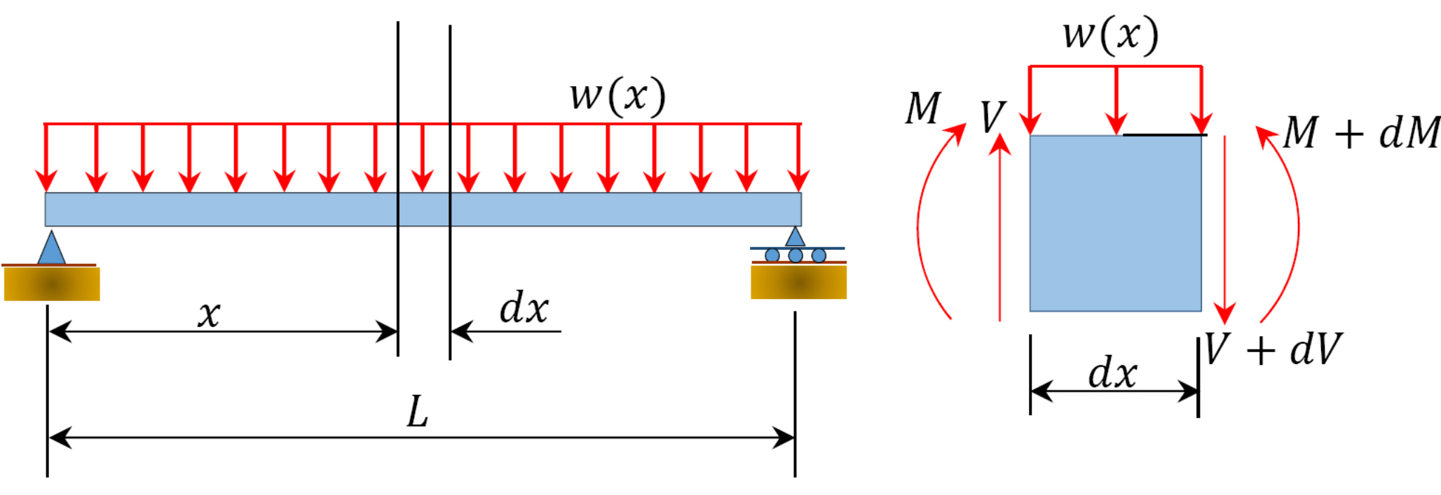
To compute the bending moment at section x + dx, use the following:
[latex]\begin{aligned} M_{x+dx} &= M + Vdx - wdx \cdot \frac{dx}{2} \\ &= M + Vdx \quad \text{(neglecting the small second order term } \frac{wdx^2}{2} \text{)} \end{aligned}[/latex]
or
[latex]\frac{dM}{dx}=V(x)[/latex] (Equation 6.1)
Equation 6.1 implies that the first derivative of the bending moment with respect to the distance is equal to the shearing force. The equation also suggests that the slope of the moment diagram at a particular point is equal to the shear force at that same point. Equation 6.1 suggests the following expression:
[latex]\Delta M=\int V(x)dx[/latex] (Equation 6.2)
Equation 6.2 states that the change in moment equals the area under the shear diagram. Similarly, the shearing force at section x + dx is as follows:
[latex]V_{x+dx}=V-wdx\\V+dV=V-wdx[/latex]
or
[latex]\frac{dV}{dx}=-w(x)[/latex] (Equation 6.3)
Equation 6.3 implies that the first derivative of the shearing force with respect to the distance is equal to the intensity of the distributed load. Equation 6.3 suggests the following expression:
[latex]\Delta V=\int w(x)dx[/latex] (Equation 6.4)
Equation 6.4 states that the change in the shear force is equal to the area under the load diagram. Equations 6.1 and 6.3 suggest the following:
[latex]\frac{d^2M}{dx^2}=-w(x)[/latex] (Equation 6.5)
Equation 6.5 implies that the second derivative of the bending moment with respect to the distance is equal to the intensity of the distributed load.
Source: Internal Forces in Beams and Frames, LibreTexts. https://eng.libretexts.org/Bookshelves/Civil_Engineering/Book%3A_Structural_Analysis_(Udoeyo)/01%3A_Chapters/1.04%3A_Internal_Forces_in_Beams_and_Frames
6.2.3 Producing a Shear/Moment Diagram
There are many methods you can use to solve a shear/moment diagram. First, you can find the equation for each portion and integrate using the above equations.
Second, you could use the method shown in the previous section to calculate the internal forces at important points (where loads are applied, the start and end of distributed loads, at reaction points). Plot these points on the V and M plots at the x locations, then connect the dots using the appropriate shape slope (more on this at the bottom of this page).
Third, you can find the equations by using the equilibrium equations (so there’s no integration/differentiation).
-
Adapted from original source https://eng.libretexts.org/Bookshelves/Civil_Engineering/Book%3A_Structural_Analysis_(Udoeyo)/01%3A_Chapters/1.04%3A_Internal_Forces_in_Beams_and_Frames Draw a FBD of the structure
- Calculate the reactions using the equilibrium equations (may not need to do this if choosing a cantilever beam and using the free side for the FBD).
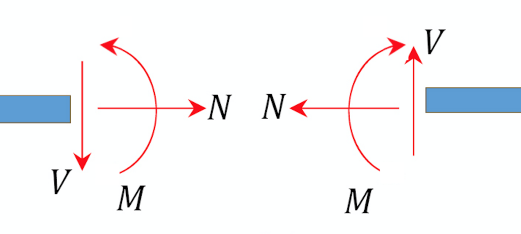
- Make a cut and add internal forces N V and M using the positive sign convention. Depending on the number of loads, you may need multiple cuts. Recall the positive convention:
- For shear, find an equation (expression) of the shear that is x distance from the origin (often the reaction) for each cut.
- For moment, find an equation (expression) of the shear that is x distance from the origin (often the reaction) for each cut.
- Plot these equations on a plot on top of each other.
The rest of this section will use this method.
Example 1
Draw the shear force and bending moment diagrams for the cantilever beam supporting a concentrated load of 5 lb at the free end 3 ft from the wall.
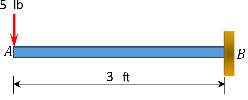
1. Draw a FBD of the structure
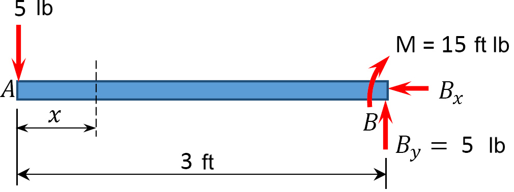
2. Calculate the reactions using the equilibrium equations (may not need to do this if choosing a cantilever beam and using the free side for the FBD).
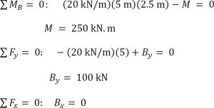
First, compute the reactions at the support. Since the support at B is fixed, there will be three reactions at that support, namely By, Bx, and MB. Applying the conditions of equilibrium suggests the following:
[latex]\sum F_{x}=0: \quad \underline{B_{x}=0}[/latex]
[latex]\sum F_{y}=0: \quad-5 lb+B_{y}=0[/latex]
[latex]\qquad \quad \underline{B_{y}=5 lb}[/latex]
[latex]\sum M_{B}=0: \quad(5 lb )(3 \mathrm{ft})-M=0[/latex]
[latex]\qquad \quad \underline{M=15 ft \cdot lb}[/latex]
3. Make a cut and add internal forces N V and M using the positive sign convention. Depending on the number of loads, you may need multiple cuts
Only 1 cut needed because only 1 load is added at the end. (If it were in the middle there would be 2 sections to consider). The value x could be 0 to 3 ft.
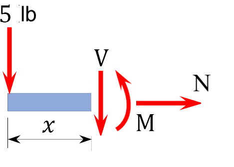
4. For shear, find an equation (expression) of the shear that is x distance from the origin (often the reaction) for each cut.
x is the distance from the free end of the cantilever beam to the cut. The shearing force at that section is due to the applied load. Using the equilibrium equations,
[latex]\sum F_y = -5 lb - V = 0 \\ \qquad \quad \underline{V = - 5 lb} \text{ (- indicates V acts in opposite direction)}[/latex]
The constant number for shear means that it doesn’t change or vary by x. (If there were a distributed load, x would be part of the equation).
The negative sign indicates the shear actually goes the opposite direction. (This is due to the fact that the sign convention for a shearing force states that a downward transverse force on the left of the section under consideration will cause a negative shearing force on that section.)
5. For the moment, find an equation (expression) of the shear that is x distance from the origin (often the reaction) for each cut.
Here, x is measured from the left. Using sum of the moments equations, find an expression for M. You could choose to sum the moments about the end point where the load is applied, or you could do it at the moving point x. Both take the same effort for this problem, so let’s choose the left hand side where the 5 lb are being applied.
[latex]\sum M_L = -Vx - M = 0[/latex]
[latex]\qquad \quad M = + Vx = (-5 lb) * x[/latex]
[latex]\qquad \quad \underline{M = -(5lb)x } \text{ (the negative sign indicates the arrow goes the other direction.}[/latex]
The obtained expression is valid for the entire beam (the region 0 < x < 3 ft). The negative sign indicates a negative moment, which was established from the sign convention for the moment, so the moment actually goes in the opposite direction. The moment due to the 5 lb force tends to cause the segment of the beam on the left side of the section to exhibit a downward concavity, and that corresponds to a negative bending moment, according to the sign convention for bending moment.
6. Plot these equations on a plot on top of each other.
Note that because the shearing force is a constant, it must be of the same magnitude at any point along the beam. As a convention, the shearing force diagram is plotted above or below a line corresponding to the neutral axis of the beam, but a plus sign must be indicated if it is a positive shearing force, and a minus sign should be indicated if it is a negative shearing force. A way to check the answer is to ensure the reaction force brings the problem back to 0. The shear is -5 until the last moment when the reaction force of +5lb brings the force to 0.
Since the function for the bending moment is linear, the bending moment diagram is a straight line. Thus, it is enough to use the two principal values of bending moments determined at x = 0 ft and at x = 3 ft to plot the bending moment diagram. As a convention, negative bending moment diagrams are plotted below the neutral axis of the beam, while positive bending moment diagrams are plotted above the axis of the beam.
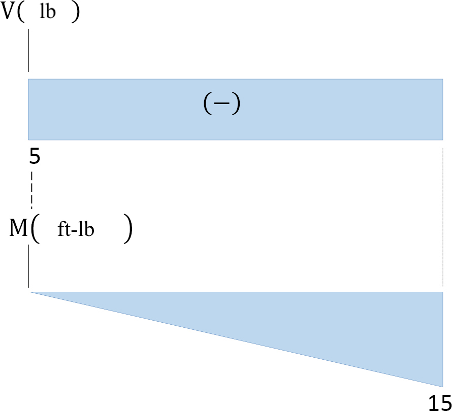
Notice the units are included in the axes.
Here is a second explanation for how to create shear/moment diagrams:
Shear Diagram
To create the shear force diagram, we will use the following process.
- Solve for all external forces acting on the body.
- Draw out a free-body diagram of the body horizontally. Leave all distributed forces as distributed forces and do not replace them with the equivalent point load.
- Lined up below the free body diagram, draw a set of axes. The x-axis will represent the location (lined up with the free body diagram above), and the y-axis will represent the internal shear force.
- Starting at zero at the right side of the plot, you will move to the right, pay attention to forces in the free body diagram above. As you move right in your plot, keep steady except…
- Jump upwards by the magnitude of the force for any point forces going up.
- Jump downwards by the magnitude of the force for any point forces going down.
- For any uniformly distributed forces, you will have a linear slope where the magnitude of the distributed force is the slope of the line (positive slopes for upwards distributed forces, negative slopes for downwards distributed forces).
- For non-uniformly distributed forces, the shape of the shear diagram plot will be the integral of the force function.
- You can ignore any moments or horizontal forces applied to the body.
By the time you get to the left end of the plot, you should always wind up coming back to zero. If you don’t wind up back at zero, go back and check your previous work.
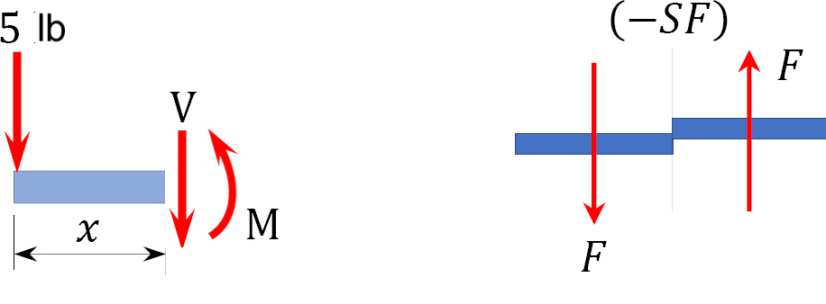
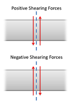 To read the plot, you simply need to find the location of interest from the free body diagram above, and read the corresponding value on the y-axis from your plot. Positive numbers represent an upward internal shearing force to the right of the cross section and a downward force on the left, and negative numbers indicate a downward internal shearing force to the right of the cross section and an upward force on the left. A visual of these forces can be seen in the diagram to the right.
Moment Diagram
The moment diagram will plot out the internal bending moment within a horizontal beam that is subjected to multiple forces and moments perpendicular to the length of the beam. For practical purposes, this diagram is often used in the same circumstances as the shear diagram, and generally, both diagrams will be created for analysis in these scenarios.
To create the moment diagram for a shaft, we will use the following process.
- Solve for all external forces and moments, create a free body diagram, and create the shear diagram.
- Lined up below the shear diagram, draw a set of axes. The x-axis will represent the location (lined up with the shear diagram and free body diagram above), and the y-axis will represent the internal bending moment.
- Starting at zero on the right side of the plot, you will move to the right, pay attention to the shear diagram and the moments in the free body diagram above. As you move right in your plot, the moment diagram will primarily be the integral of the shear diagram, except…
- Jump upwards by the magnitude of the moment for any negative (clockwise) moments.
- Jump downwards by the magnitude of the moment for any positive (counter-clockwise) moments.
- You can ignore any forces in the free body diagram.
By the time you get to the left end of the plot, you should always wind up coming back to zero. If you don’t wind up back at zero, go back and check your previous work.
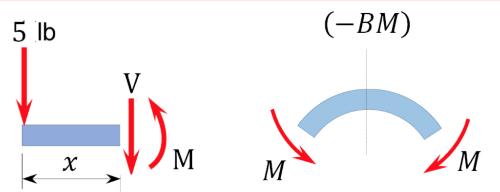
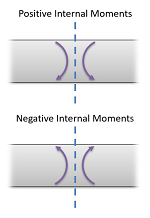 To read the plot, you simply need to take the find the location of interest from the free body diagram above, and read the corresponding value on the y-axis from your plot. Positive internal moments would cause the beam to bow downwards (think a smile shape) negative internal moments will cause the beam to bow upwards (think a frown shape). You can also see the positive and negative internal moments in the figure to the right.
Source: Engineering Mechanics, Jacob Moore, et al. http://mechanicsmap.psu.edu/websites/6_internal_forces/6-4_shear_moment_diagrams/shear_moment_diagrams.html
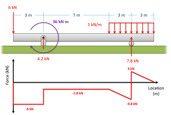
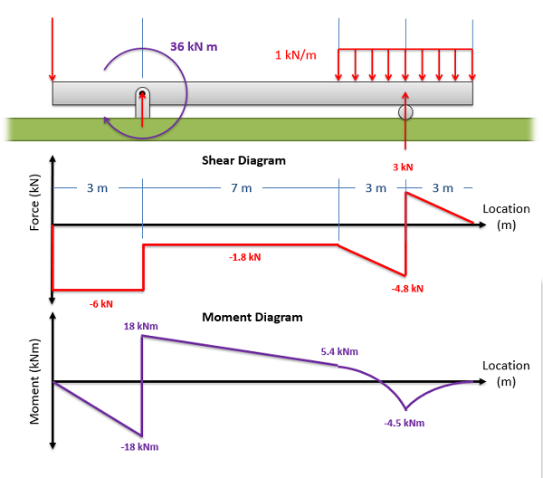
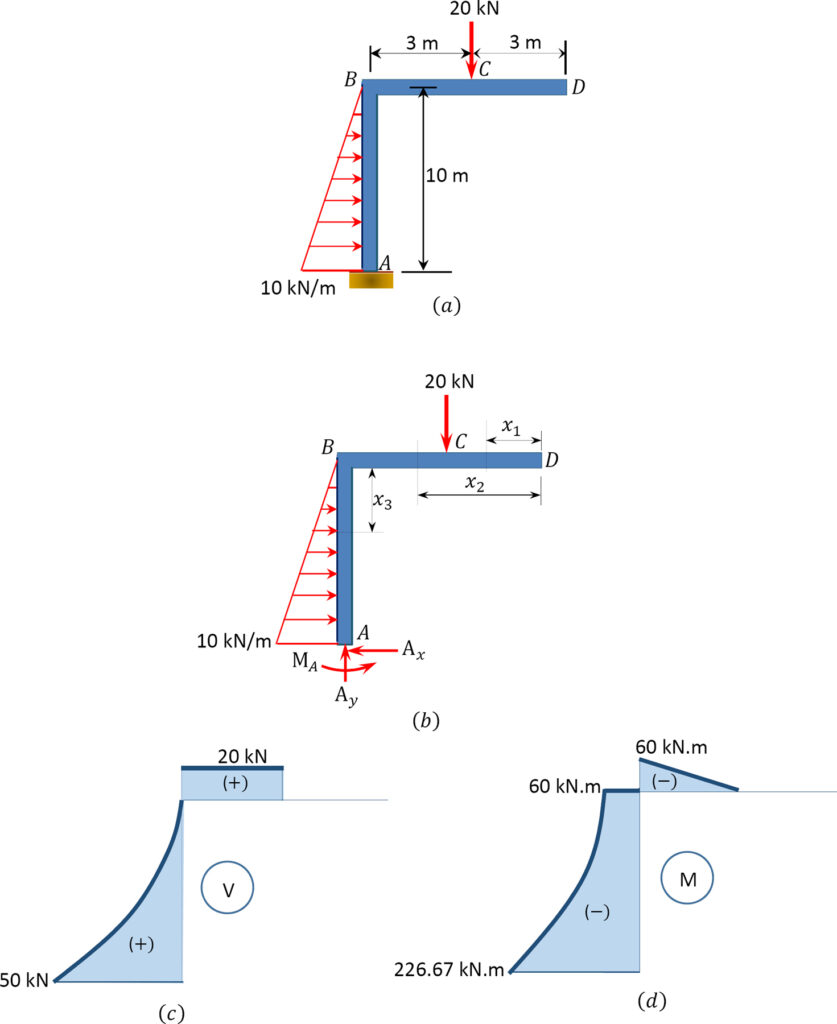
Example 2
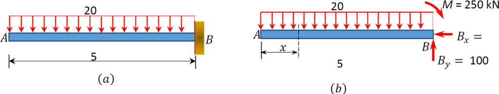
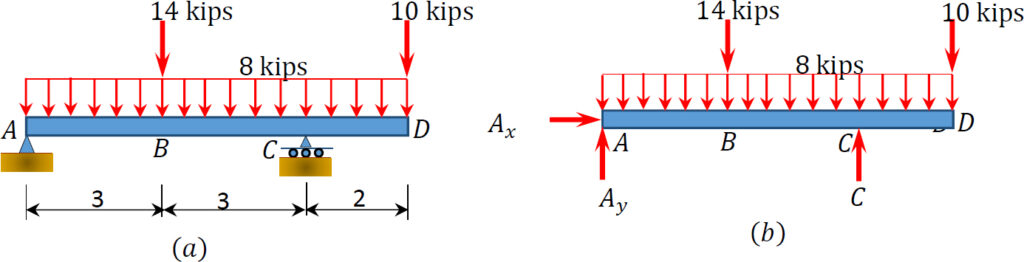
Draw the shearing force and bending moment diagrams for the cantilever beam subjected to a uniformly distributed load in its entire length, as shown in Figure 4.5a.
Answer:
Support reactions.
First, compute the reactions at the support. Since the support at B is fixed, there will possibly be three reactions at that support, namely By, Bx, and MB, as shown in the free-body diagram in Figure 4.4b. Applying the conditions of equilibrium suggests the following:
Shear Force Function
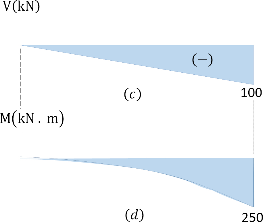
Let x be the distance of an arbitrary section from the free end of the cantilever beam, as shown in Figure 4.5b. The shearing force of all the forces acting on the segment of the beam to the left of the section, as shown in Figure 4.5e, is determined as follows:
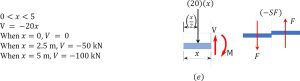 The obtained expression is valid for the entire beam. The negative sign indicates a negative shearing force, which was established from the sign convention for a shearing force. The expression also shows that the shearing force varies linearly with the length of the beam.
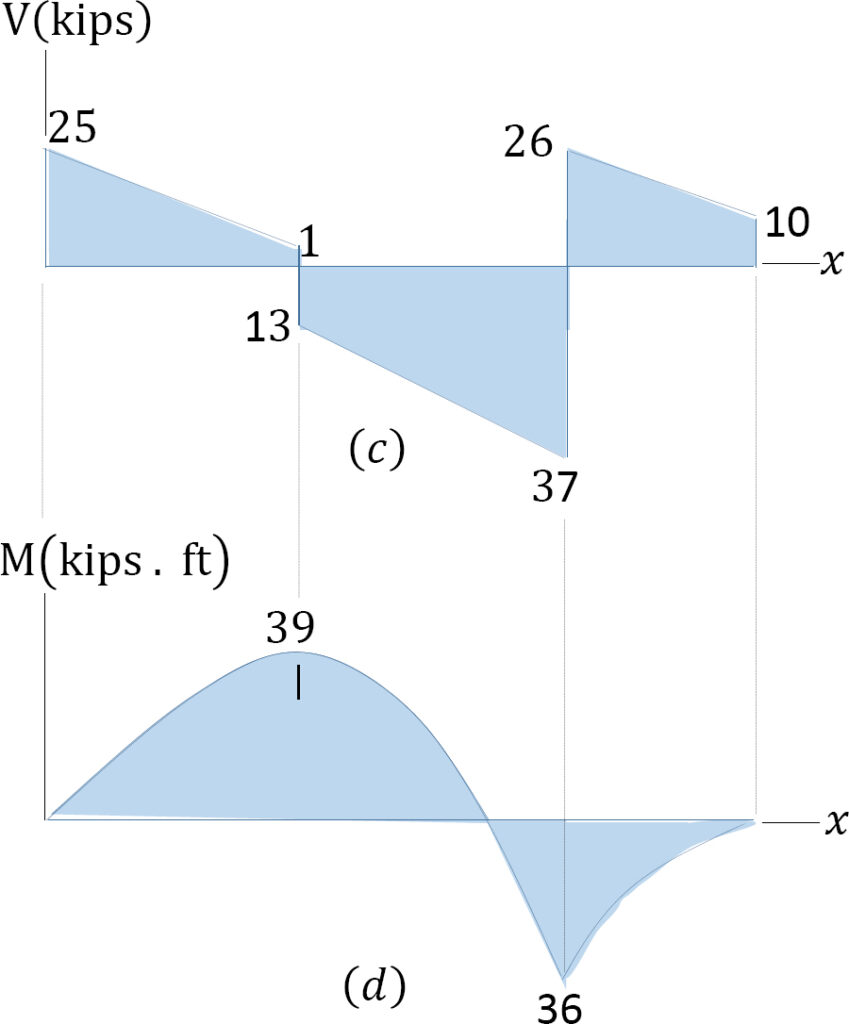
Shearing force diagram. Note that because the expression for the shearing force is linear, its diagram will consist of straight lines. The shearing forces at x = 0 m and x = 5 m were determined and used for plotting the shearing force diagram, as shown in Figure 4.5c. As shown in the diagram, the shearing force varies from zero at the free end of the beam to 100 kN at the fixed end. The computed vertical reaction of By at the support can be regarded as a check for the accuracy of the analysis and diagram.
Bending Moment Function
The expression for the bending moment at a section of a distance x from the free end of the cantilever beam is as follows:
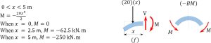 The negative sign indicates a negative moment, which was established from the sign convention for moment. As seen in Figure 4.5f, the moment due to the distributed load tends to cause the segment of the beam on the left side of the section to exhibit an upward concavity, and that corresponds to a negative bending moment, according to the sign convention for bending moment.
Bending moment diagram. Since the function for the bending moment is parabolic, the bending moment diagram is a curve. In addition to the two principal values of bending moment at x = 0 m and at x = 5 m, the moments at other intermediate points should be determined to correctly draw the bending moment diagram. The bending moment diagram of the beam is shown in Figure 4.5d.
Source: Internal Forces in Beams and Frames, Libretexts. https://eng.libretexts.org/Bookshelves/Civil_Engineering/Book%3A_Structural_Analysis_(Udoeyo)/01%3A_Chapters/1.04%3A_Internal_Forces_in_Beams_and_Frames
The following examples show the shear and moment diagrams for each beam. For details on how to solve each, go to: https://eng.libretexts.org/Bookshelves/Civil_Engineering/Book%3A_Structural_Analysis_(Udoeyo)/01%3A_Chapters/1.04%3A_Internal_Forces_in_Beams_and_Frames
Example 3
Example 4
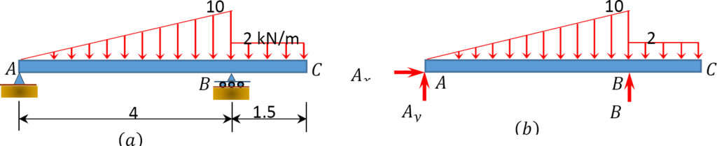
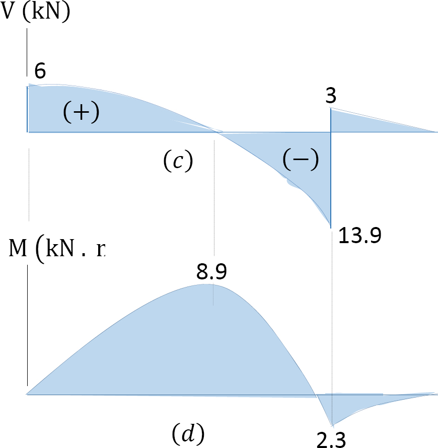
Example 5
Example 6
Source: Internal Forces in Beams and Frames, Libretexts. https://eng.libretexts.org/Bookshelves/Civil_Engineering/Book%3A_Structural_Analysis_(Udoeyo)/01%3A_Chapters/1.04%3A_Internal_Forces_in_Beams_and_Frames
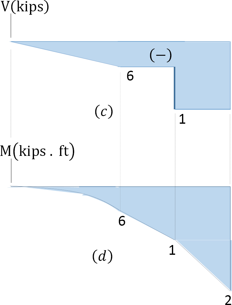
6.2.4 Tips & Plot Shapes
Though there are exceptions, these rules are generally true:
- +V means increasing M
- -V means decreasing M
- When V = 0, that’s max or min M
How does each plot start/end? Reactions only if no applied load/moment at ends:
- Cantilever:
- At start/reaction: Nonzero V and M
- At end/unsupported end: 0 for both
- Simply supported
- For V: Start and end with reaction forces
- For M: Start and end at zero
- Where are the ‘jumps’ or inflection points where lines change?
- In V, forces ‘jump’ up or down where applied forces are, matching the direction they are applied (also reactions)
- In M, moments jump up or down where applied moments are, matching the direction.
- Relationship between graphs
- When there is an increasing slope in M, then Shear should be positive
- When there is a decreasing slope in M, then Shear should be negative
- When V is positive, M should be increasing
- When V is negative, M should be decreasing
- When intensity is positive, V should be increasing
- When intensity is negative, V should be decreasing
- Inflection points in the M plot (where the slope of the line changes from negative to positive & max/min values) should be 0 in the V plot
- A zero value in the V plot should produce a max or min value in the M plot
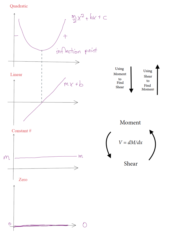
The following figure shows the relationship between the derivatives. Remember that the derivative of x2 (quadratic) = x (linear). The derivative of x (linear) is a constant number. The derivative of a constant number is 0. The derivative of the moment is shear, so if you have the shape of the moment, use this figure to approximate the shape of shear by going down the plots.
The reverse is true when going from shear to moment. The integral of shear is the moment. The integral of 0 is a constant number. The integral of a constant number is linear. The integral of a linear function is quadratic. (The integral of quadratic is cubic). This progression moves up the plots from the bottom to the top.
There are a few online programs that can help confirm the shape that you found or help you learn how to translate loads into shear and moment diagrams. These are not acceptable to use on the exam or in homework, and have limited free versions. This is not an endorsement of any of the sites, just showing learning tools.
- https://skyciv.com/free-beam-calculator/
- https://clearcalcs.com/freetools/beam-analysis/au
- https://beamguru.com/beam/
Key Takeaways
Basically: Shear / Moment diagrams graphically display the internal loads along a beam.
Application: This can help you identify the major stress points to provide a safer design.
Looking Ahead: You will use this more in your structures class.
