
Chapter 7: Inertia
7.1 Center of Mass: Single Objects
To start, let’s calculate the center of mass! This is a weighted function, similar to when we found the location of the resultant force from multiple distributed loads and forces.
[latex]\bar{x}=\frac{m_1*x_1}{m_1+m_2}+\frac{m_2*x_2}{m_1+m_2}[/latex]
When the density is the same throughout a shape, the center of mass is also the centroid (geometric center).
7.1.1 Center of Mass of Two Particles
Consider two particles, having one and the same mass m, each of which is at a different position on the x-axis of a Cartesian coordinate system.
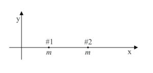
Common sense tells you that the average position of the material making up the two particles is midway between the two particles. Common sense is right. We give the name “center of mass” to the average position of the material making up a distribution, and the center of mass of a pair of same-mass particles is indeed midway between the two particles. How about if one of the particles is more massive than the other? One would expect the center of mass to be closer to the more massive particle, and again, one would be right. To determine the position of the center of mass of the distribution of matter in such a case, we compute a weighted sum of the positions of the particles in the distribution, where the weighting factor for a given particle is that fraction of the total mass that the particle’s own mass is. Thus, for two particles on the x axis, one of mass m1, at x1, and the other of mass m2, at x2,
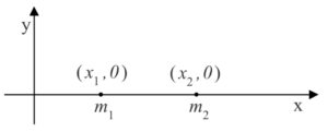
The position x of the center of mass is given by equation 8-1:
[latex]\bar{x}=\frac{m_1*x_1}{m_1+m_2}+\frac{m_2*x_2}{m_1+m_2}[/latex]
Note that each weighting factor is a proper fraction and that the sum of the weighting factors is always 1. Also note that if, for instance, m1 is greater than m2, then the position x1 of particle 1 will count more in the sum, thus ensuring that the center of mass is found to be closer to the more massive particle (as we know it must be). Further note that if m1 = m2, each weighting factor is 1/2, as is evident when we substitute m for both m1 and m2 in equation 8-1:
[latex]\bar{x}=\frac{m}{m+m}x_1+\frac{m}{m+m}x_2\\\bar{x}=\frac{1}{2}x_1+\frac{1}{2}x_2\\\bar{x}=\frac{x_1+x_2}{2}[/latex]
The center of mass is found to be midway between the two particles, right where common sense tells us it has to be.
Source: Calculus-Based Physics 1, Jeffery W. Schnick. p142, https://openlibrary.ecampusontario.ca/catalogue/item/?id=ce74a181-ccde-491c-848d-05489ed182e7
Below is a more visual representation of where the COM would be for two different weighing particles.
A second explanation:
The most common real-life example of a system like this is a playground seesaw, or teeter-totter, with children of different weights sitting at different distances from the center. On a seesaw, if one child sits at each end, the heavier child sinks down and the lighter child is lifted into the air. If the heavier child slides in toward the center, though, the seesaw balances. Applying this concept to the masses on the rod, we note that the masses balance each other if and only if m1d1 = m2d2.
This idea is not limited just to two-point masses. In general, if n masses, m1,m2,…, mn are placed on a number line at points x1, x2,…xn, respectively, then the center of mass of the system is given by:
[latex]\bar x=\frac{\sum_{i=1}^n m_i x_i}{\sum_{i=1}^nm_i}[/latex]
Example 1:
Suppose four point masses are placed on a number line as follows:
- m1 = 30kg, placed at x1 = -2m
- m2 = 5kg, placed at x2 = 3m
- m3 = 10kg, placed at x3 = 6m
- m4 = 15kg, placed at x4 = -3m
Solution
Find the moment of the system with respect to the origin and find the center of mass of the system.
First, we need to calculate the moment of the system (the top part of the fraction):
[latex]M =\sum_{i=1}^4 m_i *x_i \\\qquad \quad = (30kg)*(-2m) + (5kg)*(3m)+(10kg)*(6m)+(15kg)*(-3m) \\\qquad\quad = (-60+15+60-45)kg*m \\\qquad\quad = -30 kg*m[/latex]
Now, to find the center of mass, we need the total mass of the system:
[latex]m = \sum_{i=1}^4 m_i = (30+5+10+15) kg = 60kg[/latex]
Then we have [latex]\bar{x} = \frac{M}{m} = \frac{-30 kg*m}{60kg} = -0.5 m[/latex]
The center of mass is located 1/2 m to the left of the origin.
Source: “Moments and Centers of Mass” by LibreTexts, https://eng.libretexts.org/@go/page/67237
7.1.2 Center of Mass in 2D & 3D
When we are looking at multiple objects in 2D or 3D, we perform the center of mass equation multiple times in the x, y, and z directions.
[latex]\bar x=\frac{\sum_{i=1}^n m_i x_i}{\sum_{i=1}^nm_i} \qquad \bar y=\frac{\sum_{i=1}^n m_i y_i}{\sum_{i=1}^nm_i} \qquad \bar z=\frac{\sum_{i=1}^n m_i z_i}{\sum_{i=1}^nm_i}[/latex]
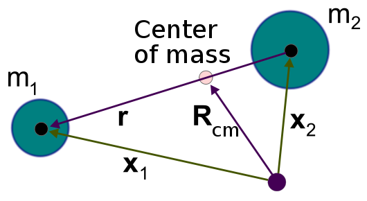
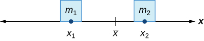
In some sense, one can think about the center of mass of a single object as its “average position.” Let’s consider the simplest case of an “object” consisting of two tiny particles separated along the x-axis, as seen below:
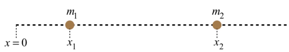
If the two particles have equal mass, then it’s pretty clear that the “average position” of the two-particle system is halfway between them. If the masses of the two particles are different, would the “average position” still be halfway between them? Perhaps in some sense this is true, but we are not looking for a geometric center; we are looking for the average placement of mass. If m1 has twice the mass of m2, then when it comes to the average placement of mass, m1 gets “two votes.” With more of the mass concentrated at the position x1 than at x2, the center of mass should be closer to x1 than x2. We achieve the perfect balance by “weighting” the positions by the fraction of the total mass that is located there. Accordingly, we define the center of mass:
[latex]\bar x_{cm}=(\frac{m_1}{m_1+m_2})x_1+(\frac{m_2}{m_1+m_2})x_2=\frac{m_1x_1+m_2x_2}{M_{system}}[/latex]
If there are more than two particles, we simply add all of them into the sum in the numerator. To extend this definition of the center of mass into three dimensions, we simply need to do the same things in the y and z directions. A position vector for the center of mass of a system of many particles would then be:
[latex]\vec{r}_{cm}=\bar x_{cm}\underline{\hat{i}}+\bar y_{cm}\underline{\hat{j}}+ \bar z_{cm}\underline{\hat{k}}\\=\frac{[m_1 x_1+m_2 x_2+...]}{M}\underline{\hat{i}}+\frac{[m_1y_1+m_2y_2+...]}{M}\underline{\hat{j}}+\frac{[m_1 z_1+m_2 z_2+...]}{M}\underline{\hat{k}}\\=\frac{m_1[x_1\underline{\hat{i}}+y_1\underline{\hat{j}}+z_1\underline{\hat{k}}]+m_2[x_2\underline{\hat{i}}+y_2\underline{\hat{j}}+z_2\underline{\hat{k}}]+...}{M}\\=\frac{m_1\vec r_1+m_2\vec r_2+...}{M}[/latex]
Source: ” Center of Mass” by Tom Weideman, https://phys.libretexts.org/Courses/University_of_California_Davis/UCD%3A_Physics_9A__Classical_Mechanics/4%3A_Linear_Momentum/4.2%3A_Center_of_Mass
Example 2:
Suppose three point masses are placed in the x-y plane as follows (assume coordinates are given in meters):
- m1 = 2 kg placed at (-1, 3)m,
- m2 = 6 kg placed at (1, 1)m, and
- m3 = 4 kg placed at (2, -2)m.
Find the center of mass of the system.
Solution
First, we calculate the total mass of the system:
[latex]m = \sum_{i=1}^3 m_i = (2 + 6 + 4) kg = 12 kg[/latex]
Next, we find the moments with respect to the x- and y-axes:
[latex]M_x =\sum_{i=1}^3 m_i *x_i \\\qquad \quad = (2kg)*(-1m) + (6kg)*(1m)+(4kg)*(2m) \\\qquad\quad = (-2+6+8)kg*m \\\qquad\quad = 12 kg*m[/latex]
[latex]M_y =\sum_{i=1}^3 m_i *y_i \\\qquad \quad = (2kg)*(3m) + (6kg)*(1m)+(4kg)*(-2m) \\\qquad\quad = (6+6-8)kg*m \\\qquad\quad = 4 kg*m[/latex]
Then we have
[latex]\bar{x} = \frac{M_x}{m} = \frac{12 kgm}{12m} = 1 m[/latex]
[latex]\bar{y} = \frac{M_y}{m} = \frac{4 kgm}{12m} = 0.333 m[/latex]
The center of mass of the system is: (1, 0.333)m.
Source: “Moments and Centers of Mass” by LibreTexts, https://eng.libretexts.org/@go/page/67237
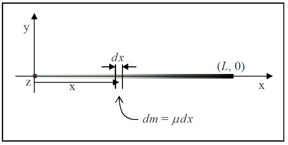
7.1.3 The Center of Mass of a Thin Uniform Rod (Calculus Method)
Quite often, when the finding of the position of the center of mass of a distribution of particles is called for, the distribution of particles is the set of particles making up a rigid body. The easiest rigid body for which to calculate the center of mass is the thin rod because it extends in only one dimension. (Here, we discuss an ideal thin rod. A physical thin rod must have some nonzero diameter. The ideal thin rod, however, is a good approximation to the physical thin rod as long as the diameter of the rod is small compared to its length.)
In the simplest case, the calculation of the position of the center of mass is trivial. The simplest case involves a uniform thin rod. A uniform thin rod is one for which the linear mass density µ, the mass per length of the rod, has one and the same value at all points on the rod. The center of mass of a uniform rod is at the center of the rod. So, for instance, the center of mass of a uniform rod that extends along the x-axis from x = 0 to x = L is at (L/2, 0).
The linear mass density µ, typically called linear density when the context is clear, is a measure of how closely packed the elementary particles making up the rod are. Where the linear density is high, the particles are close together.
To picture what is meant by a non-uniform rod, a rod whose linear density is a function of position, imagine a thin rod made of an alloy consisting of lead and aluminum. Further imagine that the percentage of lead in the rod varies smoothly from 0% at one end of the rod to 100% at the other. The linear density of such a rod would be a function of the position along the length of the rod. A one-millimeter segment of the rod at one position would have a different mass than that of a one-millimeter segment of the rod at a different position.
People with some exposure to calculus have an easier time understanding what linear density is than calculus-deprived individuals do because linear density is just the ratio of the amount of mass in a rod segment to the length of the segment, in the limit as the length of the segment goes to zero. Consider a rod that extends from 0 to L along the x-axis. Now, suppose that ms(x) is the mass of that segment of the rod extending from 0 to ,x where x ≥ 0 but x < L. Then, the linear density of the rod at any point x along the rod is just dm8/dx evaluated at the value of x in question.
Source: Calculus-Based Physics 1, Jeffery W. Schnick. p143, https://openlibrary.ecampusontario.ca/catalogue/item/?id=ce74a181-ccde-491c-848d-05489ed182e7
7.1.4 The Center of Mass of a Non-Uniform Rod
Now that you have a good idea of what we mean by linear mass density, we are going to illustrate how one determines the position of the center of mass of a non-uniform thin rod by means of an example.
Example 3:
Find the position of the center of mass of a thin rod that extends from 0 to 0.890 m along the x-axis of a Cartesian coordinate system and has a linear density given by µ = 0.650 kg/m3
In order to be able to determine the position of the center of mass of a rod with a given length and a given linear density as a function of position, you first need to be able to find the mass of such a rod. To do that, one might be tempted to use a method that works only for the special case of a uniform rod, namely, to try using m = µL with L being the length of the rod. The problem with this is that µ varies along the entire length of the rod. What value would one use for µ? One might be tempted to evaluate the given µ at x = L and use that, but that would be acting as if the linear density were constant at µ = µ(L). It is not. In fact, in the case at hand, µ(L) is the maximum linear density of the rod; it only has that value at one point on the rod.
Instead, using integration, we find the equation:
[latex]m=\frac{bL^3}{3}[/latex]
That can now be used to calculate the mass of a nonlinear rod. The value of L is given as 0.890 m, and we defined b to be the constant 0.650 kg/m3, therefore
[latex]m=\frac{0.650\frac{kg}{m^3}(0.890m)^3}{3}\\m=0.1527kg[/latex]
That’s a value that will come in handy when we calculate the position of the center of mass.
Now, when we calculated the center of mass of a set of discrete particles (where a discrete particle is one that is by itself, as opposed, for instance, to being part of a rigid body) we just carried out a weighted sum in which each term was the position of a particle times its weighting factor and the weighting factor was that fraction, of the total mass, represented by the mass of the particle. We carry out a similar procedure for a continuous distribution of mass such as that which makes up the rod in question.
Once again, using integration, we find the equation:
[latex]\bar{x}=\frac{bL^4}{4m}[/latex]
Now we substitute variables with values; the mass m of the rod that we found earlier, the constant b that we defined to simplify the appearance of the linear density function, and the given length L of the rod:
[latex]m= \frac{\left( 0.650\frac{kg}{m^3} \right) (0.890m)^4}{4(0.1527kg)}\\\bar{x}=0.668m[/latex]
This is our final answer for the position of the center of mass. Note that it is closer to the denser end of the rod, as we would expect.
Source: Calculus-Based Physics 1, Jeffery W. Schnick. p144, https://openlibrary.ecampusontario.ca/catalogue/item/?id=ce74a181-ccde-491c-848d-05489ed182e7
Key Takeaways
Basically: When there are multiple objects, the center of mass is the location in the x, y, and z directions between the objects.
Application: To calculate the acceleration or use F = ma, m is the total mass at the center of mass.
Looking Ahead: The next section will look at how to calculate the center of mass for a complex object.
