
Chapter 3: Rigid Body Basics
3.3 Distributed Loads
3.3.1 Intensity
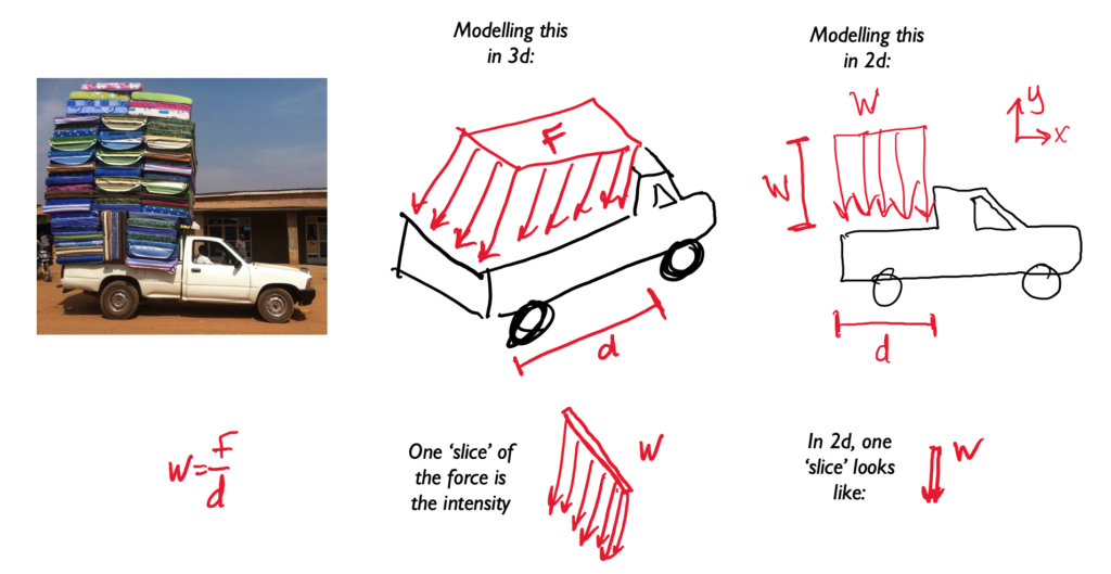
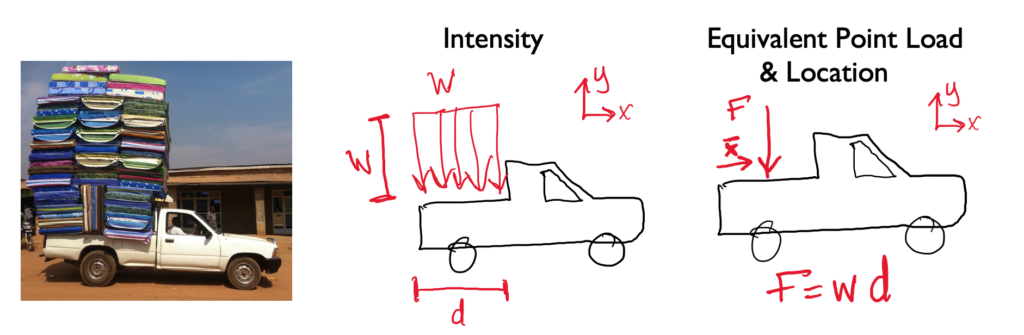
Distributed loads are a way to represent a force over a certain distance. Sometimes called intensity, given the variable:
Intensity w = F / d [=] N/m, lb/ft
While pressure is force over area (for 3d problems), intensity is force over distance (for 2d problems). It’s like a bunch of mattresses on the back of a truck. You can model it as 1 force acting at the center (an equivalent point load as in 3.3.2, or you can model it as intensity and divide the total force by the width of the truck bed (the distance that’s not visible in this image[1]).
A distributed load is any force where the point of application of the force is an area or a volume. This means that the “point of application” is not really a point at all. Though distributed loads are more difficult to analyze than point forces, distributed loads are quite common in real-world systems, so it is important to understand how to model them.
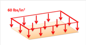
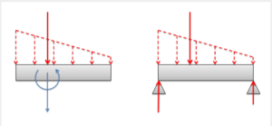
Distributed loads can be broken down into surface forces and body forces. Surface forces are distributed forces where the point of application is an area (a surface on the body). Body forces are forces where the point of application is a volume (the force is exerted on all molecules throughout the body). Below are some examples of surface and body forces.


Distributed loads are represented as a field of vectors. This is drawn as a number of discrete vectors along a line, over a surface, or over a volume, that are connected with a line or a surface, as shown below.
Though these representations show a discrete number of individual vectors, there is actually a magnitude and direction at all points along the line, surface, or body. The individual vectors represent a sampling of these magnitudes and directions.
It is also important to realize that the magnitudes of distributed forces are given in force per unit distance, area, or volume. We must integrate the distributed load over its entire range to convert the force into the usual units of force.
Analyzing Distributed Load:
For analysis purposes in statics and dynamics, we will usually substitute in a single point force that is statically equivalent to the distributed load in the problem. This single point force is called the equivalent point load and it will cause the same accelerations or reaction forces as the distributed load while simplifying the math.
Source: Engineering Mechanics, Jacob Moore et al., http://mechanicsmap.psu.edu/websites/4_statically_equivalent_systems/4-4_distributed_forces/distributedforces.html
An additional example:
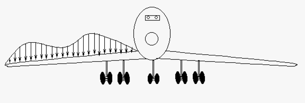 This is a more complex example of a distributed load. This is a cartoon of an airplane with its wing covered in a combination of snow and ice. In a real-world situation, loads will not accommodate people for ease of calculation; you get what you get. In this case, we could approximate this shape with two semi-circles on each end of the wing with a triangle [latex]\nabla[/latex] in the middle. For more accuracy, we could use a system similar to the trapezoidal rule.
Source: ” Statics” by LibreTexts is licensed under CC BY-NC-SA. https://eng.libretexts.org/Bookshelves/Introduction_to_Engineering/EGR_1010%3A_Introduction_to_Engineering_for_Engineers_and_Scientists/14%3A_Fundamentals_of_Engineering/14.11%3A_Mechanics/14.11.01%3A_Statics
3.3.2 Equivalent Point Load & Location
Distributed loads can be modelled as a single point force that is located at the centroid of the object. You can use straightforward algebra, or use integration for more complex shapes. Then you replace the distributed load with the single point load acting at x distance. See the truck example:
There are two ways to calculate this, using integrals and using the area and centroid.
An equivalent point load is a single point force that will have the same effect on a body as the original loading condition, which is usually a distributed load. The equivalent point load should always cause the same linear acceleration and angular acceleration as the original load it is equivalent to (or cause the same reaction forces if the body is constrained). Finding the equivalent point load for a distributed load often helps simplify the analysis of a system by removing the integrals from the equations of equilibrium or equations of motion in later analysis.
Finding the Equivalent Point Load
When finding the equivalent point load we need to find the magnitude, direction, and point of application of a single force that is equivalent to the distributed load we are given. In this course we will only deal with distributed loads with a uniform direction, in which case the direction of the equivalent point load will match the uniform direction of the distributed load. This leaves the magnitude and the point of application to be found. There are two options available to find these values:
- We can find the magnitude and the point of application of the equivalent point load via integration of the force functions.
- We can use the area/volume and the centroid/center of volume of the area or volume under the force function.
The first method is more flexible, allowing us to find the equivalent point load for any force function that we can make a mathematical formula for (assuming we have the skill in calculus to integrate that function). The second method is usually faster, assuming that we can look up the values for the area or volume under the force curve and the values for the centroid or center of volume for the area under the curve.
Using Integration in 2D Surface Force Problems:
Finding the equivalent point load via integration always begins by determining the mathematical formula that is the force function. The force function mathematically relates the magnitude of the force (F) to the position (x). In this case the force is acting along a single line, so the position can be entirely determined by knowing the x coordinate, but in later problems we may also need to relate the magnitude of the force to the y and z coordinates. In our example below, we can relate magnitude of the force to the position by stating that the magnitude of the force at any point in Newtons per meter is equal to the x position in meters plus one.
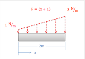
The magnitude of the equivalent point load will be equal to the area under the force function. This will be the integral of the force function over its entire length (in this case, from x = 0 to x = 2).
[latex]F_{eq}=\int_{xmin}^{xmax}F(x)dx[/latex]
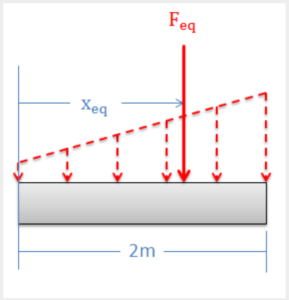
Now that we have the magnitude of the equivalent point load such that it matches the magnitude of the original force, we need to adjust the position (xeq) such that it would cause the same moment as the original distributed force. The moment of the distributed force will be the integral of the force function (F(x)) times the moment arm about the origin (x). The moment of the equivalent point load will be equal to the magnitude of the equivalent point load that we just found times the moment arm for the equivalent point load (xeq). If we set these two things equal to one another and then solve for the position of the equivalent point load (xeq), we are left with the following equation:
[latex]x_{eq}=\frac{\int_{xmin}^{xmax}(F(x)\ast x)dx}{F_{eq}}[/latex]
Now that we have the magnitude, direction, and position of the equivalent point load, we can draw the point load in our original diagram. This point force can be used in place of the distributed force in further analysis.
Using the Area and Centroid in 2D Surface Force Problems:
As an alternative to using integration, we can use the area under the force curve and the centroid of the area under the force curve to find the equivalent point load’s magnitude and point of application, respectively.
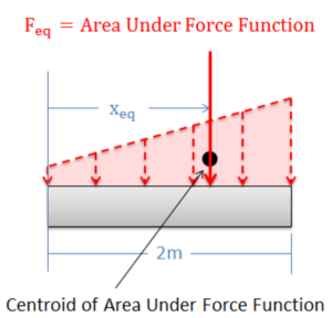
The magnitude(Feq) of the equivalent point load will be equal to the area under the force function. We can find this area using calculus, but there are often easier geometry-based ways of finding the area under the force function.
The equivalent point load will also travel through the centroid of the area under the force function. This allows us to find the value for xeq. The centroid for many common shapes can be looked up in tables, and the parallel axis theorem can be used to determine the centroid of more complex shapes (see the centroid page for more details).
Source: Engineering Mechanics, Jacob Moore et al., Mechanics Map – Equivalent Point Load via Integration
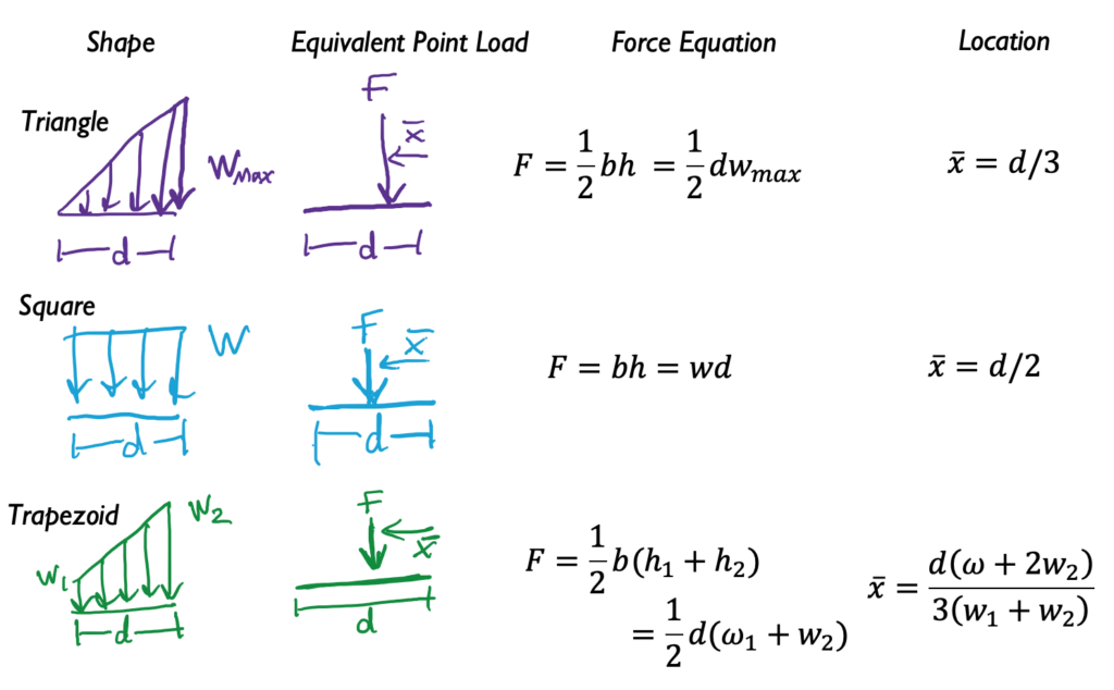
Here are the equations for some common shapes:
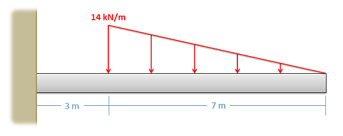
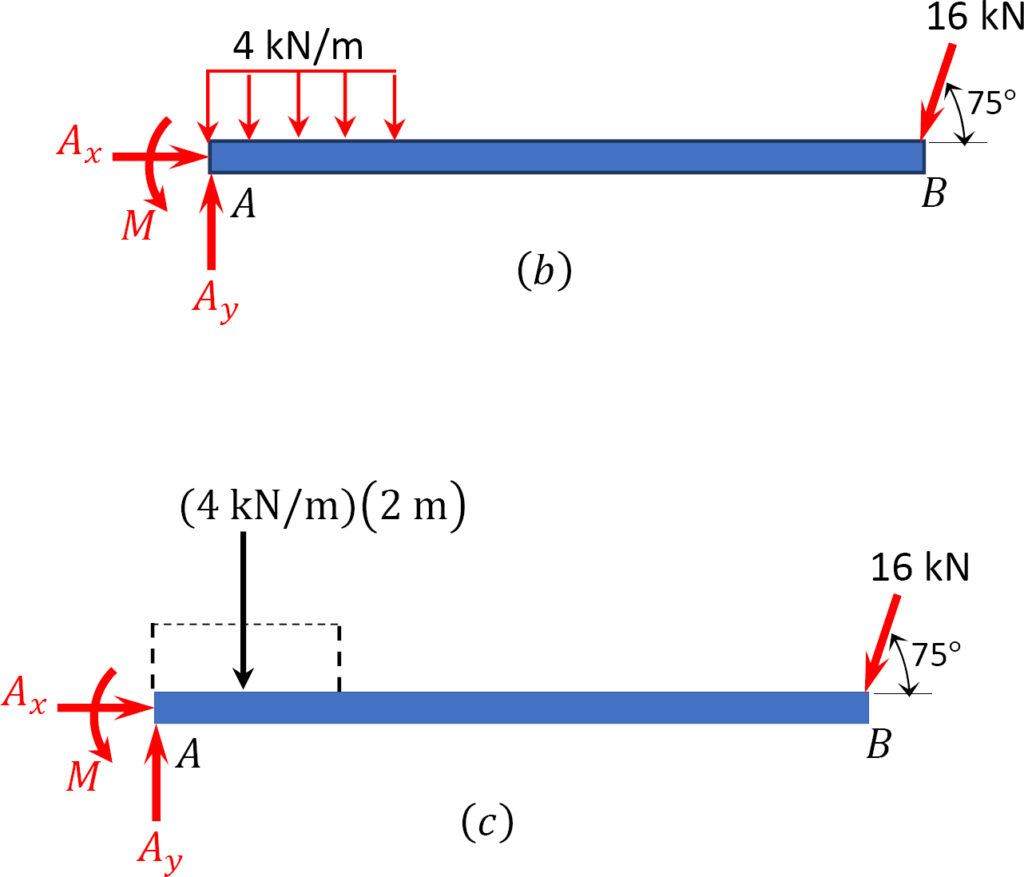
 Example 1: Equivalent force and location:
What is the resultant force and where does it act from the wall?
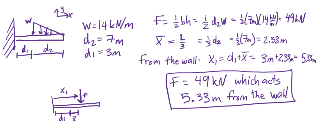
See solution here using integration from Engineering Mechanics, Jacob Moore et al., https://mechanicsmap.psu.edu/websites/4_statically_equivalent_systems/4-5_equivalent_point_load_integration/pdf/P1.pdf
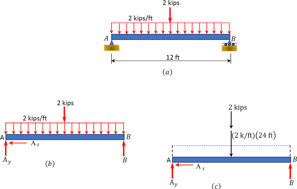
Example 2 (note: 1 kip = 1000 lb):
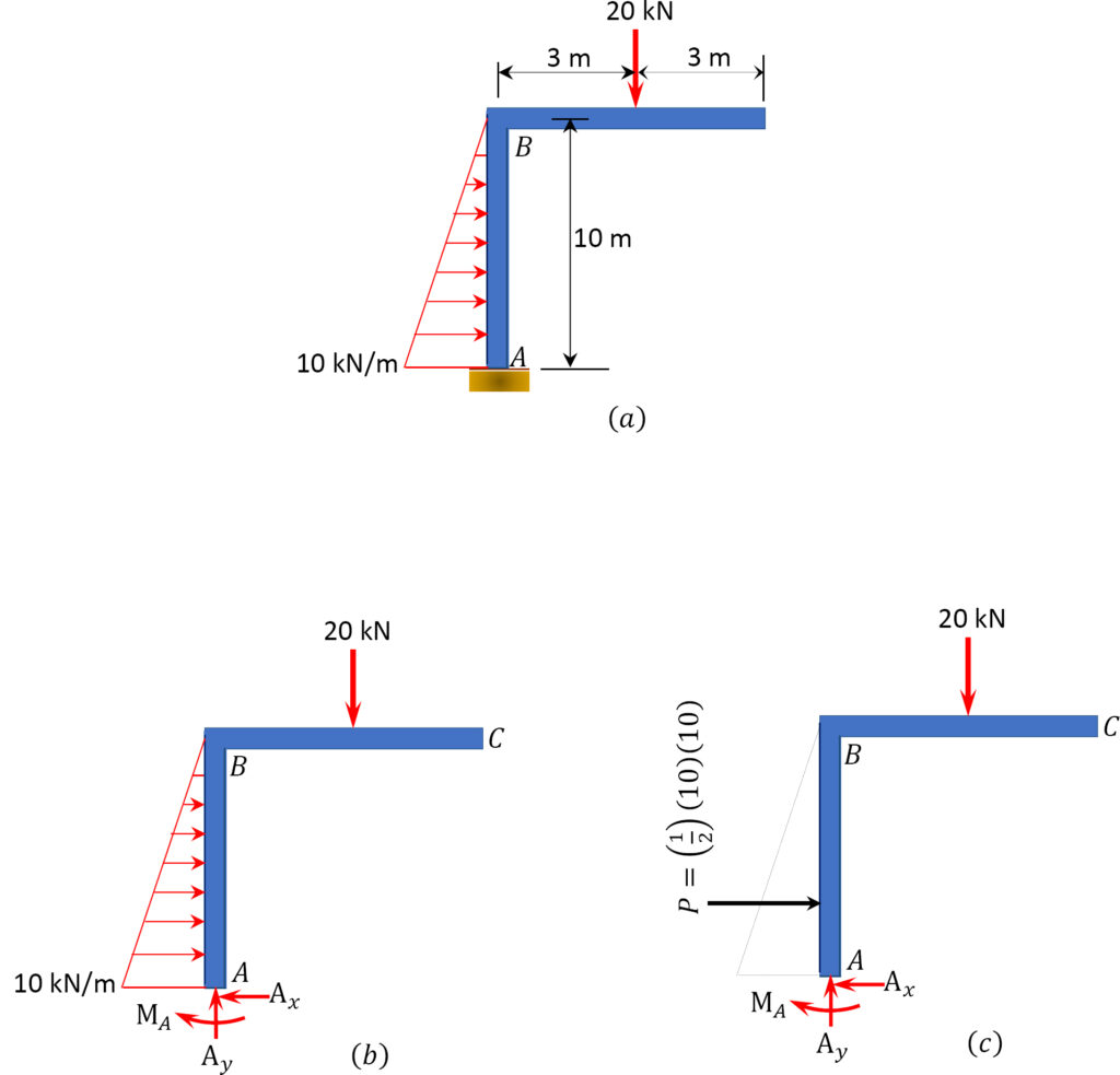
Example 3:
Example 4:
Source: ” Equilibrium Structures, Support Reactions, Determinacy and Stability of Beams and Frames” by LibreTexts is licensed under CC BY-NC-ND . https://eng.libretexts.org/Bookshelves/Civil_Engineering/Book%3A_Structural_Analysis_(Udoeyo)/01%3A_Chapters/1.03%3A_Equilibrium_Structures_Support_Reactions_Determinacy_and_Stability_of_Beams_and_Frames
3.3.3 Composite Distributed Loads
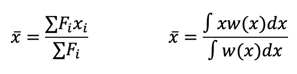
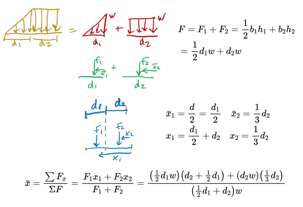
When there is a complicated shape, it can be easier to model it as more than 1 type of distributed load. You calculate each force separately and then use a weighted equation to find the total distance the force acts from a point that you select.
[latex]\quad\quad\quad\quad\text{Using area: }\quad\quad\quad\quad\quad\quad\quad\quad\quad \text{Using Integrals:}\\ \quad\quad\quad\quad\bar{x}=\frac{\sum F_{i}x_i}{\sum F_i} \quad\quad\quad\quad\quad\quad\quad\quad\quad\quad \bar{x}=\frac{\int x w(x) d x}{\int w(x) d x}[/latex]
A bit bigger:
For the following complex shape, this is how you find the composite equivalent point force and location ([latex]\bar{x}[/latex]):
Key Takeaways
Basically: Distributed loads are a way to model forces in 2d. F = w d. Sometimes called intensity, distributed loads have units of force over distance: N/m or lb/ft.
Application: For a truck carrying a heavy, uneven load, find where the center of the force is.
Looking ahead, Distributed load helps to model uneven loads. We’ll see it again as we do the beam analysis
- Image of truck from: https://get.pxhere.com/photo/car-transport-truck-vehicle-market-mattress-full-load-small-business-rwanda-overload-pickup-truck-overfull-automobile-make-612534.jpg ↵
