Chapter 3: Georeferencing in QGIS
Stream B: Georeferencing a Map of Georgetown from 1880
Downloads
We will acquire the 1880 map of Georgetown from the Island Imagined website. Island Imagined is part of the Island Archives network of websites, which are run in large part by the Island Archives Centre at the University of Prince Edward Island.
- Click here to access the map on the Island Imagined website.
- For Windows users, right-click on the map and click “Save as”
- Save the image as a PNG image
- If that doesn’t work, you may download the Georgetown map directly here.
Instructions for downloading the map on the old website
- To download the highest resolution copy of the map, do not zoom in to the map using the “plus” button in the top-left, as shown in this screenshot:
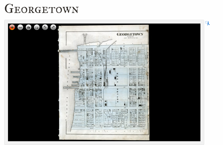
- Instead, leave the image zoomed out and click the scissors icon shown in the top right of the screenshot above.
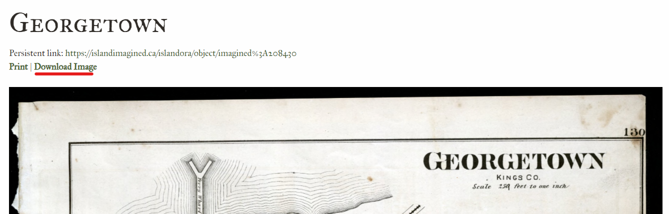
- A new page will load, where you can click Download Image. The image will download as a JPEG.
- Note: Make sure to download your image to the Rasters subfolder that we created earlier.
Georeferencing
Preparing the GIS for Georeferencing
- Make sure that you have the OpenStreetMap layer added to your QGIS project.
- Also make sure that it is the only layer that is visible. You may have to uncheck any other layers.
- Make sure your project’s coordinate reference system is set to EPSG:2954.
Preparing the Images for Georeferencing
To georeference in QGIS, we will use a tool called the Georeferencer.
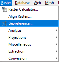
- Enter the Georeferencer tool. On Windows this tool can usually be accessed via the Raster menu.
- On Mac versions of QGIS 3.22 and older, the Georeferencer tool is under Raster, but on some versions, including QGIS 3.23, the Georeferencer tool is found under the Layer menu.
This will open the Georeferencer window.
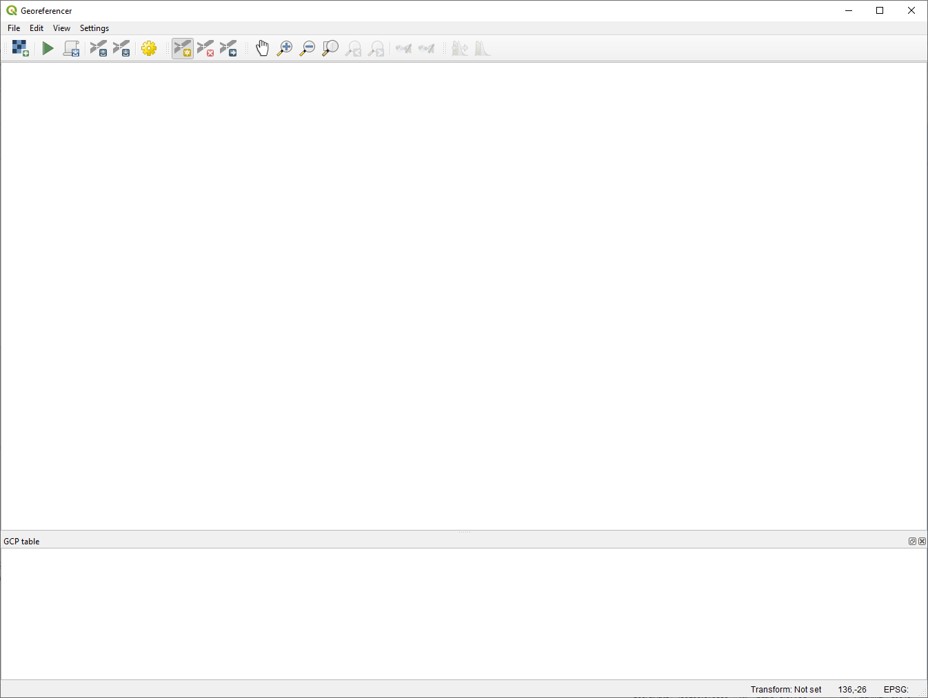
Next, we will add the raster of the map we want to georeference.
- Click this symbol to add the raster of Meacham’s map of Georgetown.

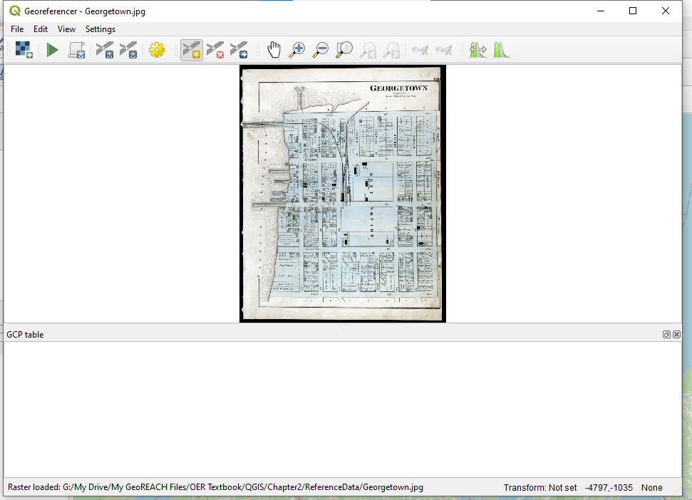
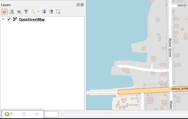
- To return to the Main Canvas (where our OpenStreetMap is), click the minimize button on the Georeferencer window.
Preparing the Basemap for Georeferencing
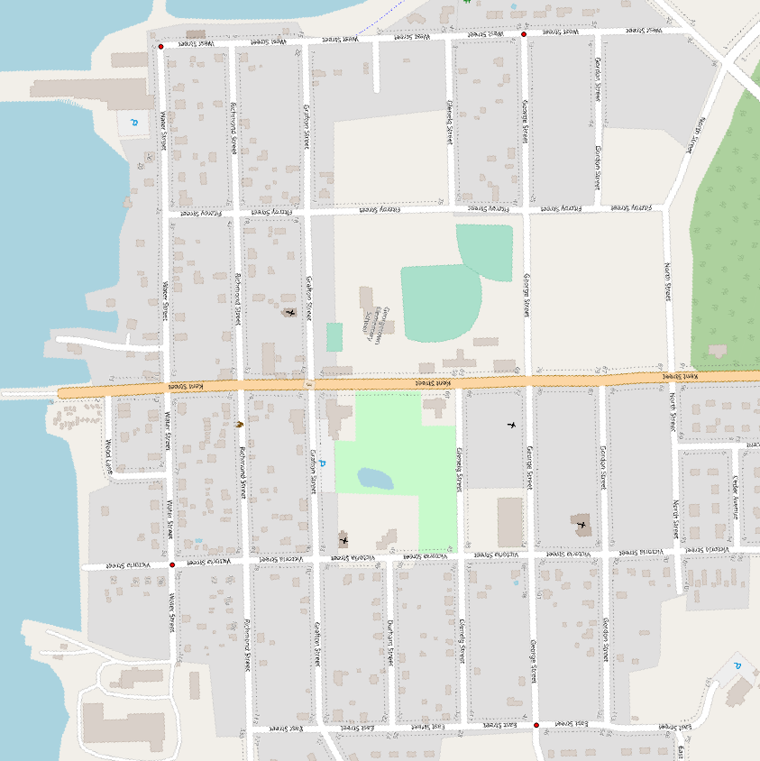
- Zoom in on the OpenStreetMaps layer to Georgetown, Prince Edward Island.
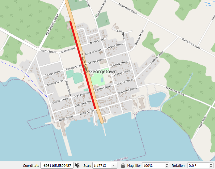
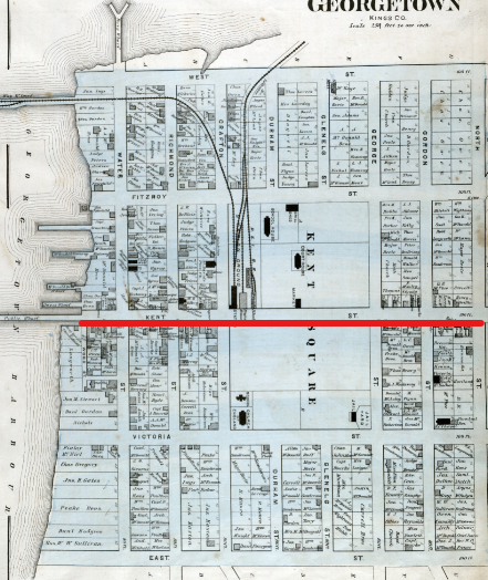
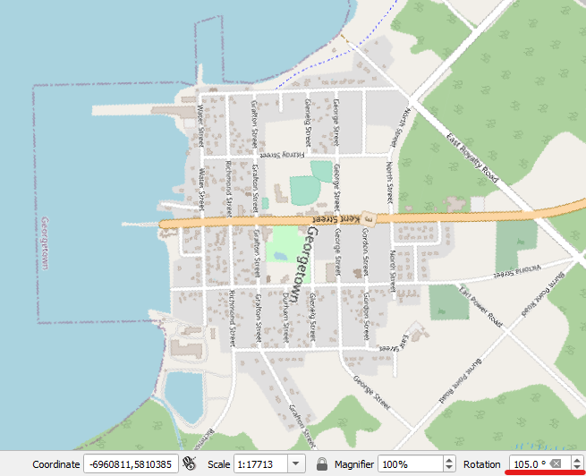
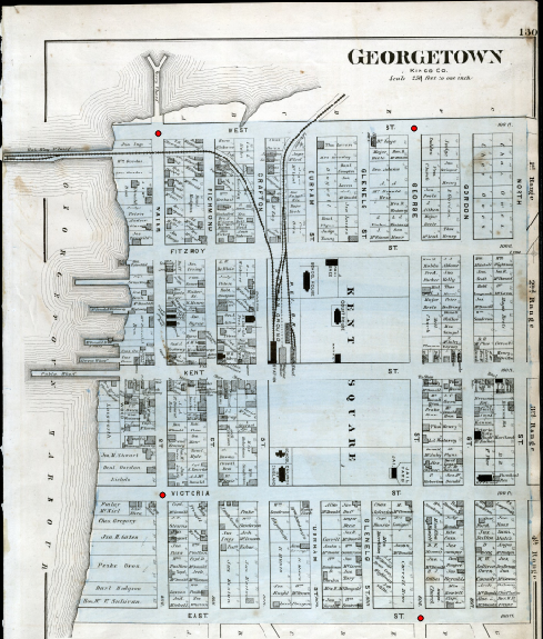
In the OpenStreetMaps map, Georgetown’s Kent Street is running almost vertically up and down our display. But, in the Meacham’s Atlas image, Kent Street is running horizontally.
It will be easier to identify common elements between the two maps if we reorient the OpenStreetMaps map to match the orientation of the Meacham’s Atlas map. To do so:
- Change the Rotation of the OpenStreetMaps map to 105.0°
Adding Control Points
What Are Control Points?
Now that we have added the map to the Georeferencer tool, we will start adding control points. These control points are points on the historical map that exist on a modern map—in this case, the OpenStreetMaps layer.
Adding control points is the means by which users precisely align the raster map with the reference map. A “control point” is actually made up of two sub-points—one that users place on the raster map and one that they place on the reference map. When you place these two points, you are telling QGIS that these two points represent the same geographic location.
At the end of the georeferencing process, after you have placed your control points, QGIS will know how to align the historical image with the modern-day map. It will align the raster image so that the control sub-point you placed on it is positioned directly above the corresponding control sub-point you placed on the reference map.
QGIS’ Control Point Buttons
The following buttons on the toolbar represent, from left to right,
![]()
- Add Control Point
- Delete Control Point
- Move Control Point
Adding Control Points
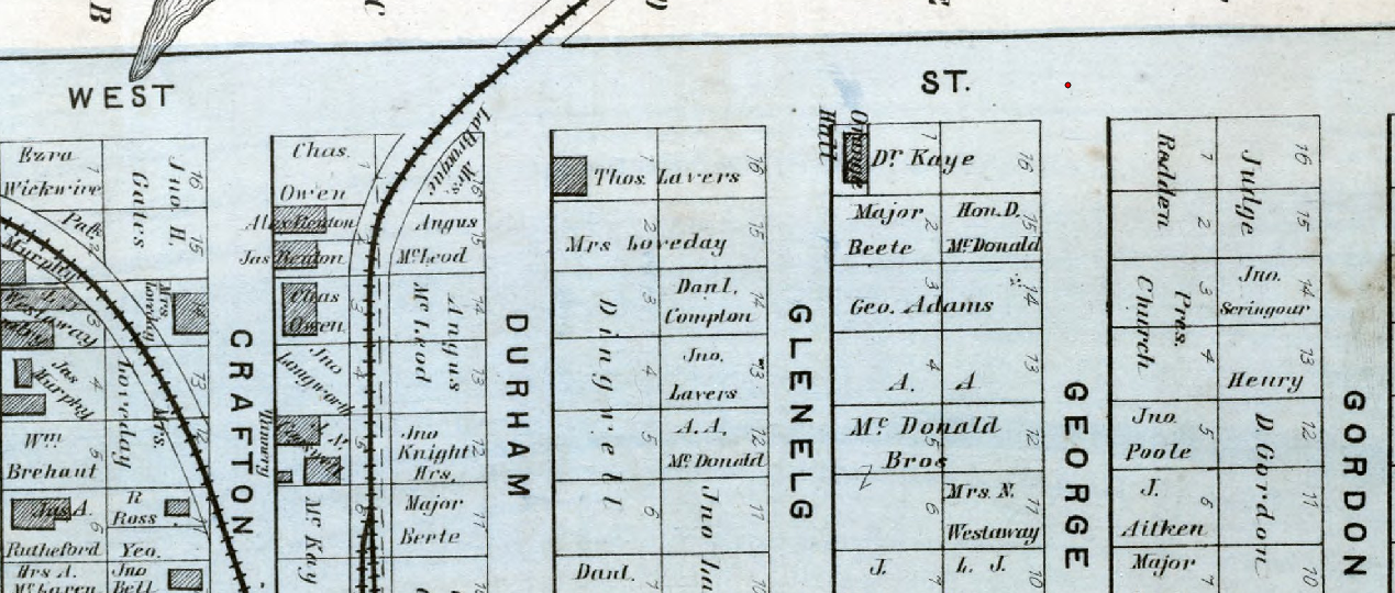
Before we can add control points, we need to look at our map of Georgetown from 1880 and our OpenStreetMap of Georgetown.
- Visually identify the geographic features that are clearly common between these two maps.
These features are often political borders and boundaries, buildings, street intersections, and bridges.
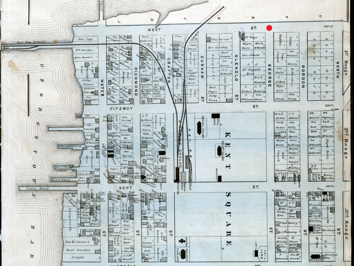
An urban map, the plan of Georgetown focuses on streets, buildings, and town blocks. While some of Georgetown’s features have changed between 1880 and today, its distinctive grid-pattern layout has remained largely unaltered. Considering this consistency in street layout between the 1880 and modern-day maps, it seems like using street intersections for control points would produce an accurate georeference.
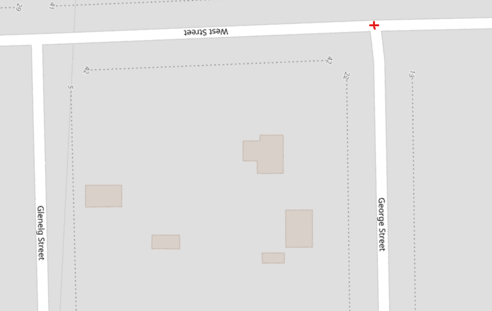
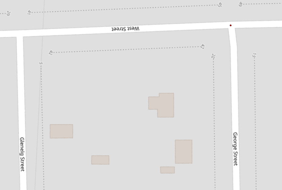
It seems that the intersection between West St. and George St. would be a good spot to place our first control point.
Now that we have identified a street intersection that aligns between the 1880 map and the OpenStreetMap,
- In the Georeferencer window, click Add Control Point
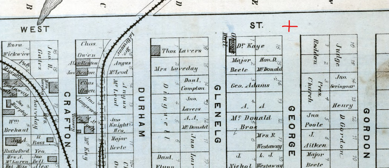
- Your cursor will now turn into crosshairs.
- Click in the very middle of the intersection between West St. and George St. in the 1880 map.
With these principles of control point placement in mind, we must consider the conventions and intentions of the 1880 map. It was an urban map with a focus on street and building locations, and it was intended for use at the town or regional scale. In other words, it was not intended as a property map or as a tool to guide municipal surveyors or developers.
In this case, urban historians usually choose the middle of a street or intersection as the most accurate control point. This is in case there are markings on the historical map that were meant to indicate edge features (eg. sidewalks) that were very likely to change as road infrastructure changed over time.
Once you place the first control subpoint on the 1880 map, the “Enter Map Coordinates” window will pop up:
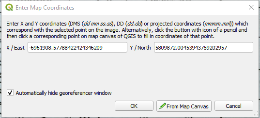
- Click “From Map Canvas”
Upon clicking this, the georeferencer window will minimize itself to the bottom-left of your screen underneath your table of contents. If you ever need to reopen the Georeferencer window, you can click its “maximize” button.
In the main QGIS window,
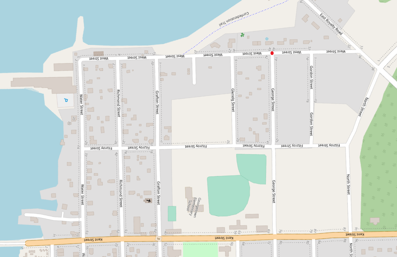
- Click in the very middle of the intersection between West St. and George St. in the OpenStreetMap.
After you click on the OpenStreetMap, the “Enter Map Coordinates” window will reappear within the Georeferencer. The X / East and Y / North coordinates will now be filled in.
- Click OK.
Once you have placed a control point, it will appear as a red dot on the historical map in the Georeferencer window and on the modern-day map in the main QGIS window.
If you happen to make a mistake while adding a control point, you can delete it.
- In the Georeferencer window, click Delete Point

- Your cursor will turn into crosshairs. Click on the red control point you wish to delete, and it will be deleted.
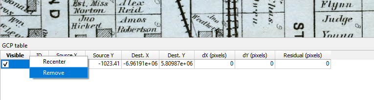
At the bottom of the Georeferencer window, there is a “GCP Table,” which lists the control points that you have added. As an alternate way of deleting a control point, you can right-click a control point in this table and click “Remove.”
You can now repeat the steps in the “Adding Control Points” section until your raster is completely georeferenced. Generally speaking, in order to completely georeference a raster of a historical map, one will usually add a minimum of four and a maximum of ten control points.
It is helpful to spread out your control points across the map, and it is usually best to try to place one control point in each of the corners of the image.
Four control points—especially if placed in the four corners of the historical map—can quickly orient the raster into the correct position in relation to the reference map. Although you may place more than ten control points, after you have placed ten, any further points you place will have an increasingly diminished effect on the orientation of the historical map in relation to the reference map. This Georgetown map from 1880 can be georeferenced fairly accurately with four control points, one on each of its four corners:
If, during the process of adding control points, your work goes totally askew, you can erase all of your control points, remove the raster, and restart. To do so,
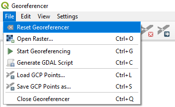
- In the Georeferencer window, click File and then Reset Georeferencer
Saving Control Points
Before continuing, we can save our control points to a .points file for future use. This can be helpful if we need to re-georeference the same map and we wish to reload our control points. Or we can use these control points again in a different future project.
To save your control points,
- Click Save GCP Points

- Save your control points in the ControlPoints subfolder within the Chapter3 folder. Name the control points file “GeorgetownControlPoints”
If you ever wish to load control points,
- Click Load GCP Points

Transformation Settings
Before we can complete the georeferencing process, we need to select a Transformation type.
Transformation is the equation by which QGIS “transforms” the raster to its real map coordinates. Every time you georeference a raster, it goes through a transformation to reach its real-world coordinates. Transformation settings determine how QGIS interprets your control points while georeferencing your raster. The Transformation process affects the scale, rotation, and precision of the map data.
The transformation settings can be viewed and set by clicking the Transformation Settings button in the Georeferencer window:
![]()
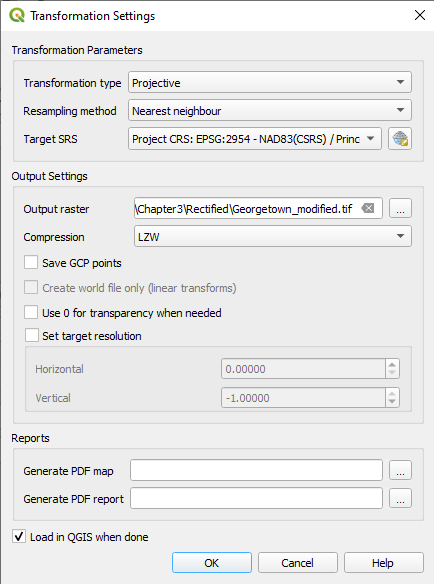
We need to specify a Transformation Type, Resampling Method, Target SRS, and Compression. We also need to provide an Output Raster name.
Transformation Types
There are several types of transformations that QGIS uses to place the raster dataset accurately onto its reference map. Listed as least to most complex, these types are Linear, Helmert, three types of Polynomial, Thin Plate Spline, and Projective. Generally, the more complex a transformation type, the more control points that are required.
The Linear transformation type is the simplest. It does not alter the raster. Helmert will alter the raster by altering its position on the X/Y/Z axes, altering its scale, and altering is rotation.
The Polynomial transformations are some of the most commonly used transformations among GIS users. They can warp the raster, which can be key when georeferencing scanned images of old maps that do not always align exactly with the base map. Among the three polynomial transformation options, Polynomial 1 will change the raster the least. Polynomial 1 will keep lines on the raster straight, but it will change the angles between them. It will also adjust the scale and rotation of your raster. Polynomial 2 and Polynomial 3 are used when you need to alter your raster more drastically. Polynomial 2 will begin to bend straight lines, and Polynomial 3 bends them to a greater extent.
Thin Plate Spline is a rather complex transformation. It allows for local areas of an image to have their own independent warping. For example, one part of an image might rotate one direction, while another part of the image might rotate in an entirely different direction. Because they have their own warping, these local areas will be very accurate at the expense of global accuracy.
The Projective transformation is useful when georeferencing scanned maps, especially if you are concerned with having accurate local data. The Projective transformation can warp lines to make them straight.
For a more detailed explanation of QGIS’ various transformation types, please see Chapter 7: Advanced Georeferencing and Digitization.
Choosing a Transformation Type
We are working with Georgetown, a town built in a square grid. We may not wish to distort these straight lines, so it seems that the Projective transformation option is perhaps the best fit for our project. This transformation type requires four control points, and we have placed four.
- Click Projective in the Transformation Type dropdown menu.
Resampling Method
Resampling is the process of taking an amount of data as a sample and calculating the precision of the data, based on the sample. Smoothing data refers to removing irregularities, such as small sudden spikes, based on the sample.
The following options are available in QGIS for resampling:
- Nearest Neighbour
- Linear
- Cubic
- Cubic Spline
- Lanczos
If you select Nearest Neighbour, few changes will be made to your raster. However, the Lanczos option makes the most changes to your raster to smooth it out as much as possible. Each resampling method between Nearest Neighbour and Lanczos delivers a progressively smoother result.
It does not seem that our project requires a great deal of smoothing out. So, Nearest Neighbour seems to be a good fit.
- Select Nearest Neighbour from the Resampling Method dropdown menu.
Target SRS
The Target SRS should match your Project CRS. If you will recall, our Project CRS is 2954.
- Select EPSG: 2954 from the Target SRS dropdown menu.
Output Raster
Here is where we can choose where we would like to save our georeferenced raster. The default location that QGIS gives is the same location where the original raster was stored. However, we would like to save our georeferenced rasters to the Rectified subfolder within the Chapter3 folder.
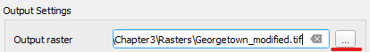
- Click Browse.
- Navigate to the Rectified subfolder within the Chapter3 folder and click Save.
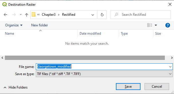
QGIS automatically appends “_modified” to the existing raster file’s name.
Compression
Compression is heavily dependent on hardware and processing power. The purpose of compression is to make the output file smaller. If a compressed file is “lossless,” the compression process has not degraded its quality. By contrast, if a compressed file is “lossy,” the compression process has degraded the file’s quality in order to significantly reduce the file’s size.
The following compression options are available in QGIS:
- LZW (Lempel-Ziv-Welch) is a lossless compression algorithm commonly used for GIFs and TIF files.
- PACKBITS is a fast and simple lossless compression algorithm.
- DEFLATE is a lossless data compression algorithm commonly used in archives.
It seems that LZW will do the trick.
- Select LZW from the Compression dropdown menu.
Load in QGIS When Done
Before clicking OK in the Transformation Settings window, we can select “Load in QGIS when done.” When we click this, QGIS will automatically load the georeferenced raster into our project without us having to click Layer and then Add Layer from the top menu in QGIS.
- Check the box in the Transformation Settings window that is called “Load in QGIS when done.”
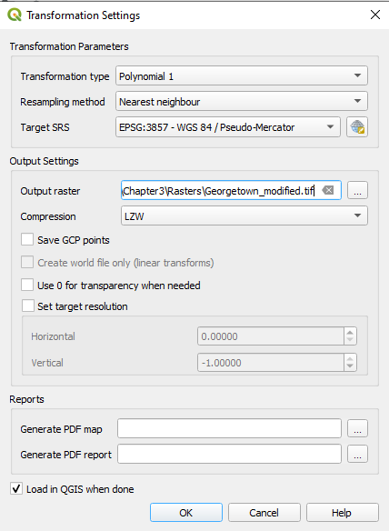
When all of your settings reflect the ones selected in the following screenshot, you can click OK to close the Transformation Settings window:
Completing the Georeferencing Process
Once we have configured our transformation settings, we can complete the georeferencing process. To do so,
- Click the Start Georeference Button
![]()
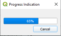
This will open a small Progress Bar that will represent the progress of your georeferencing process. Once it has reached 100%, you will have your georeferenced raster added to your Project and saved in your Rectified folder.
Once the georeference is complete, you will receive this message:

You can now close the Georeferencer window. Your map has been georeferenced.
Checking the Accuracy of the Georeferenced Map
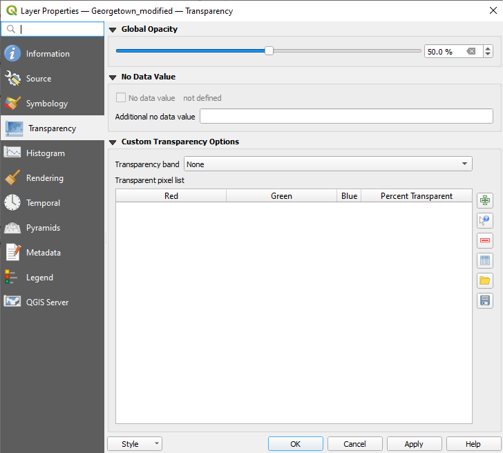
As we did with the 1991 NTS map of Georgetown, we can adjust the transparency of the 1880 map of Georgetown in order to see how well it aligns with the base map.
- Right-click the 1880 Georgetown map in the table of contents.
- Click Properties
- Click Transparency
- Change the Global Opacity to 50%.
- Click OK.
- Zoom into the Georgetown area.
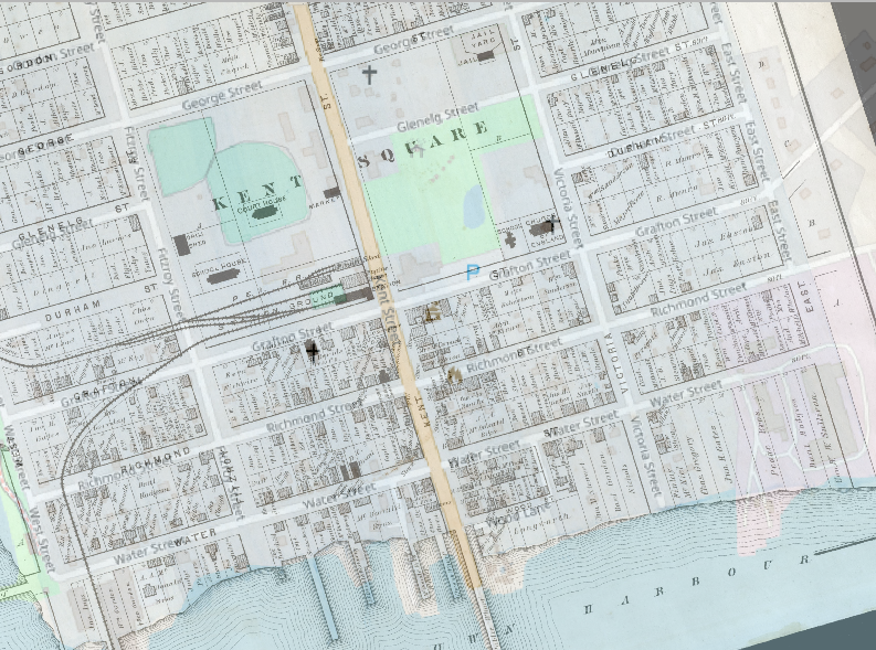
- Compare the streets in the 1880 Georgetown map with those in the underlying OpenStreetMaps base map. How well do they align?
As we can see in the screenshot below, the 1880 map of Georgetown and the OpenStreetMaps layer align very well. Almost all of the streets, including Kent Street and Richmond Street, align almost exactly. We can now be confident that our georeferencing is accurate.