
Chapter 4: Digitization in QGIS
Stream A: Creating Vectors from a Basemap and an NTS Map
Mapping a “Ghost Town”
In Stream A, we will create points, lines, and polygons. We will create points for St. David’s Presbyterian Church, the Holy Trinity Anglican Church, and the King’s Playhouse. By mapping these points, we can show which structures were in place in Georgetown in 1991.
In Stream A, we will also digitize the main road leading into Georgetown (i.e., Kent Street) as a line. We will also digitize Kent Square as a polygon.
By completing Stream A, you will learn how to create all three types of vector data. You will see the few things that Georgetown, a “ghost town,” still has to offer.
Creating Vectors: Points, Lines, and Polygons
Points
Creating a New Shapefile Layer
The first type of vector data that we will create is point data. As you will recall from the beginning of this chapter, vector data comes in the form of a shapefile. So, to create our vector data, we will first create a new shapefile layer. To do so,
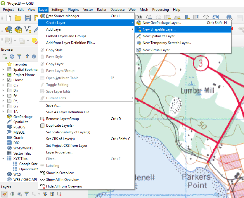
- Click Layer
- Hover over Create Layer
- Click New Shapefile Layer
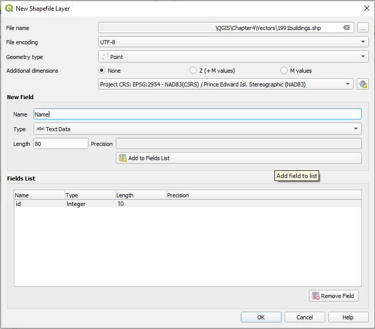
Fill out the following information in the dialogue box that appears:
File Name: …QGIS\Chapter4\Vectors\1991buildings.shp
- First, you will have to create the folder named “Vectors” inside Chapter4. This should only have to happen once in this tutorial.
- To create the Vectors folder and save the shapefile in the correct location, click the ellipsis (. . .) to the right of the File Name field.
- Navigate to QGIS\Chapter4 folder.
- Click “New Folder” and name the folder Vectors
- Enter 1991buildings as a File Name, and then click Save.
File Encoding: UTF-8
Geometry Type: Point
Additional Dimensions: None
Underneath Additional Dimensions, we can also make sure the CRS is set to “Project CRS: EPSG: 2954.”
Under New Field, we can enter the following information:
- Name: Name
- Type: TextString (in some versions “Text Data”)
We can leave the other settings.
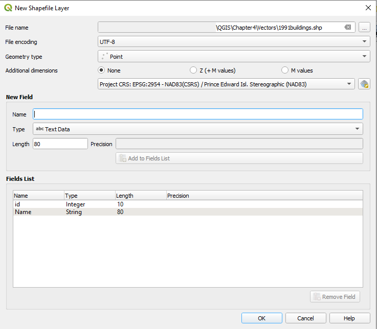
- Click Add to Fields List.
We are creating this new field so that we can keep track of the names of the places for which we are creating points.
- Click OK
Adding Points to the Reference Map
An Important Note about Scale
Before we add our points, we must take a moment to think about the scale of the NTS map. A point’s accuracy decreases as the scale of the map decreases. The NTS map of Georgetown to which we will be adding our points was created to show the region around Georgetown and not to show Georgetown itself. In other words, it is a small-scale map, and it is not an urban map. When you add a point to a small-scale map, it will not be as accurate as if you added a point to a large-scale map.
In all forms of historical research, there are limitations. In our case, the scale of the NTS map limits us. We can use the NTS map to see a fairly accurate indication of where we should place a point, but we will have to use the modern-day basemap in conjunction with the NTS map to verify the point’s proper location.
To do this, we first must be sure that the object that we are trying to represent with a point—e.g., a building—is still there on the basemap and has not changed location. We then identify the building on the NTS map. Before we commit to placing our point on the building’s location on the NTS map, we verify the location of the point on the basemap. So, in other words, the NTS map is indicating to us a building’s general location, and the basemap, which is set at a larger scale, is confirming the building’s precise location. We will make our final decision as to where to place our point based on the location of the building on the basemap.
The small scale of the NTS map is important to keep in mind when working with it alone, as we are doing in Stream A. We want to use the basemap to make sure that the points we are adding are accurate. But the NTS map’s scale is doubly important for users who will be completing Stream B. In Stream B, we work with the 1880 Meacham’s Map of Georgetown, which is at a much larger scale. It is an urban map. So, in order to accurately compare points between the 1991 and 1880 maps, we must make sure that we used the same scale when mapping each.
Adding the Points
Now that we have our new shapefile created and we have the scale of the NTS map in mind, we can start to add our points to our 1991 map of Georgetown.
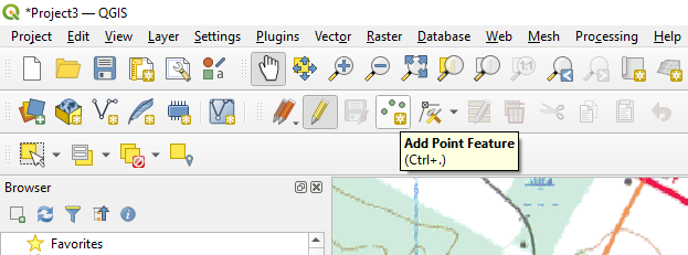
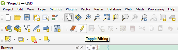
- Click Toggle Editing
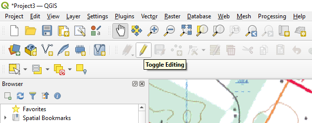
- Click Add Point Feature
Adding a Point for St. David’s Presbyterian Church
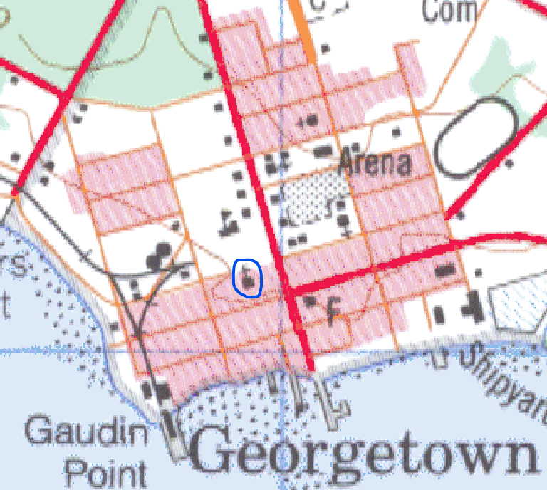
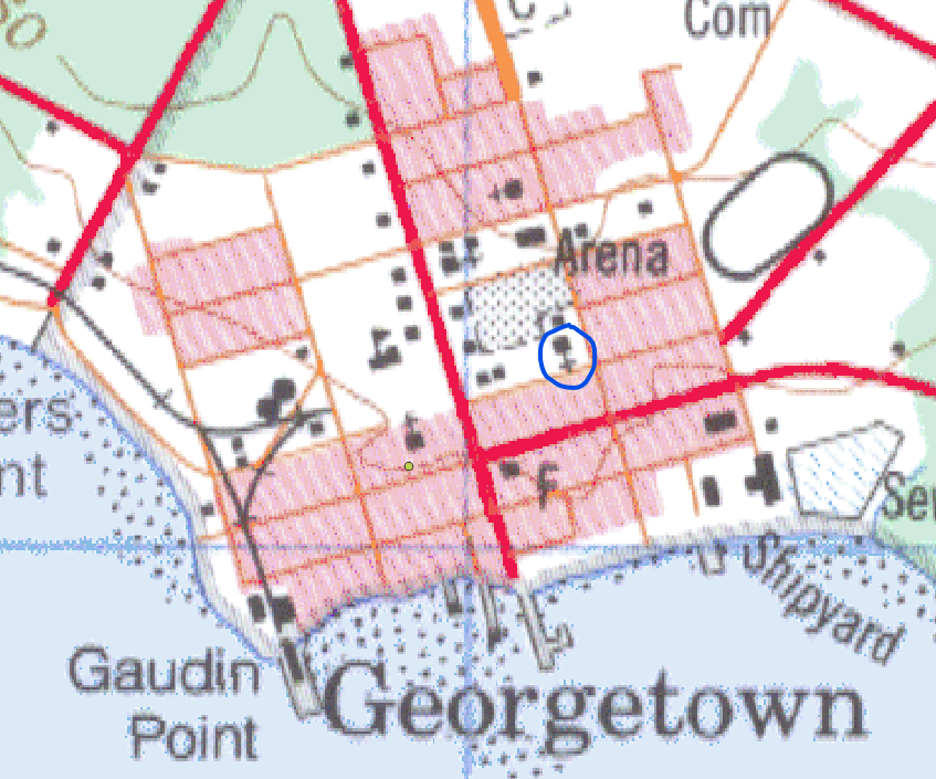
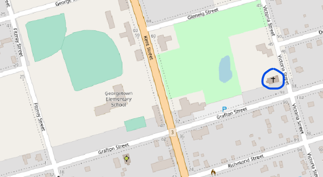
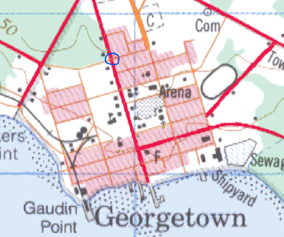
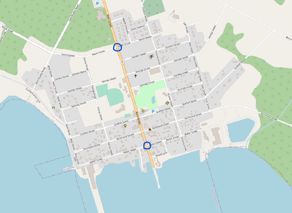
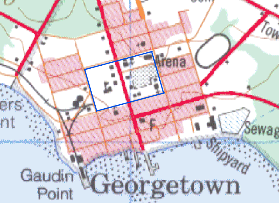
- Identify St. David’s Presbyterian Church. It is not named in the NTS map, but you will likely be able to find it by looking at the screenshot below. Its icon is drawn with a cross, and it is circled in blue in the screenshot.
- Before you place a point on this location on the NTS map, turn off the NTS map in QGIS’ Table of Contents and turn on the OpenStreetMaps basemap. Use the basemap to verify the church’s location. The church is represented on the basemap with a cross as well.
- You might have to zoom in a little to see the OpenStreetMap clearly. But this is a good thing, for, by making our scale larger, we are ensuring the point’s accuracy.
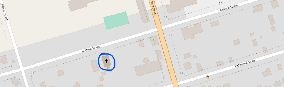
- Click on the location of the church on the OpenStreetMap to place our point.
- In the Feature Attributes dialogue box that appears, type in the following details:
- ID: 01
- As we add more points to the 1991buildings layer, we will give each new point a unique ID number.
- Name: St. David’s Presbyterian Church
- ID: 01
- Click OK.
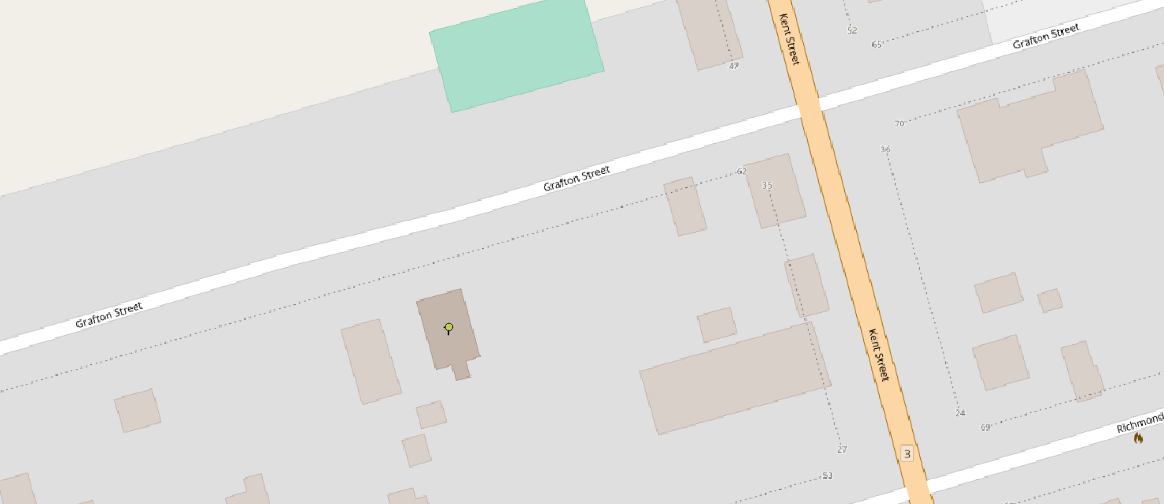
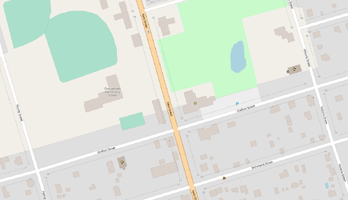
You will now see a point appear where St. David’s Presbyterian Church is on the basemap. In my case, the point is green.
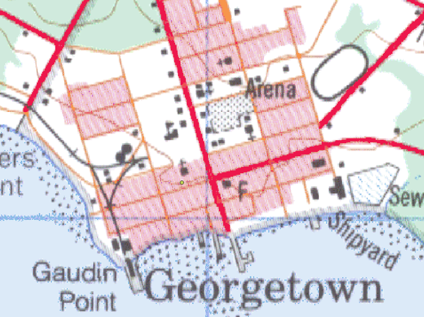
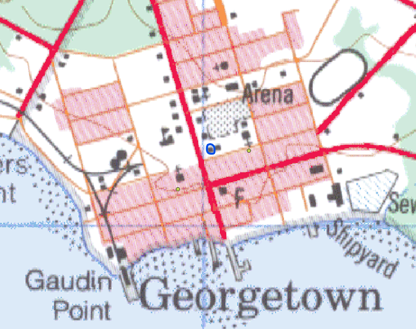
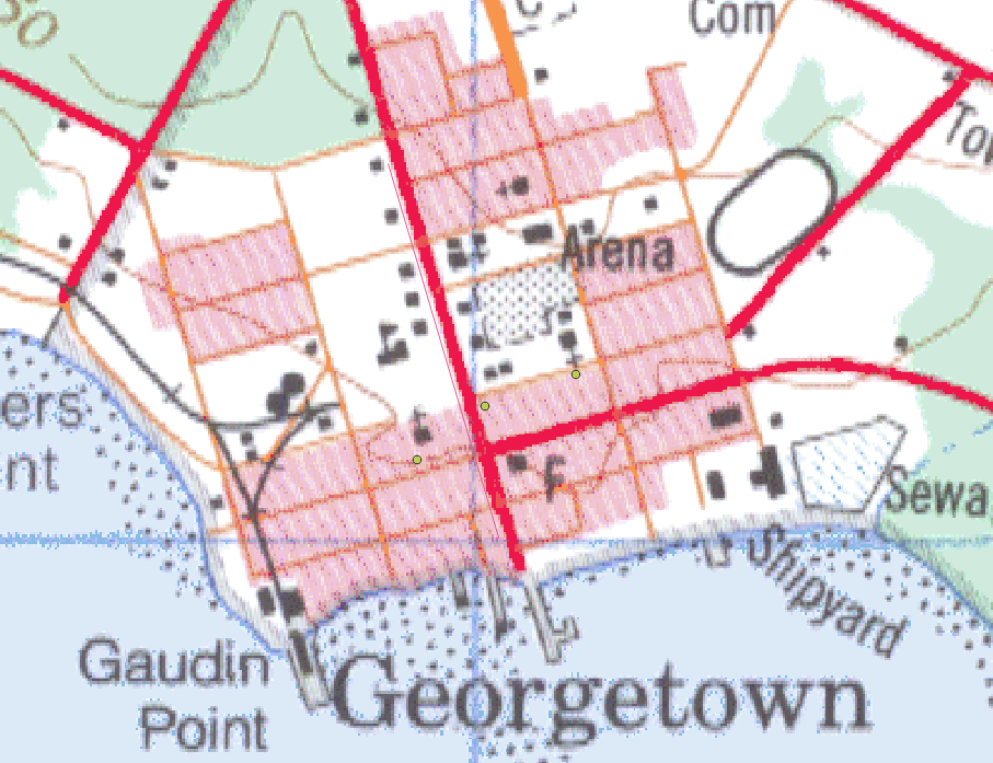
Since we used the basemap to decide the final location of the point, let’s have a look at the location of the church on the NTS map to see how much more accurate we made our point’s location by using the basemap.
As we can see in the following screenshot, the small scale of the NTS map makes its representation of the church’s location a bit inaccurate. We ensured that our point was as accurate as possible by using the basemap.
Adding a Point for the Holy Trinity Anglican Church
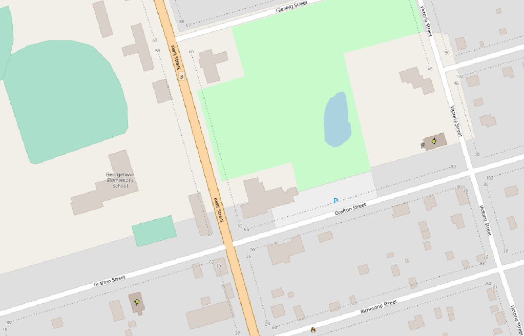
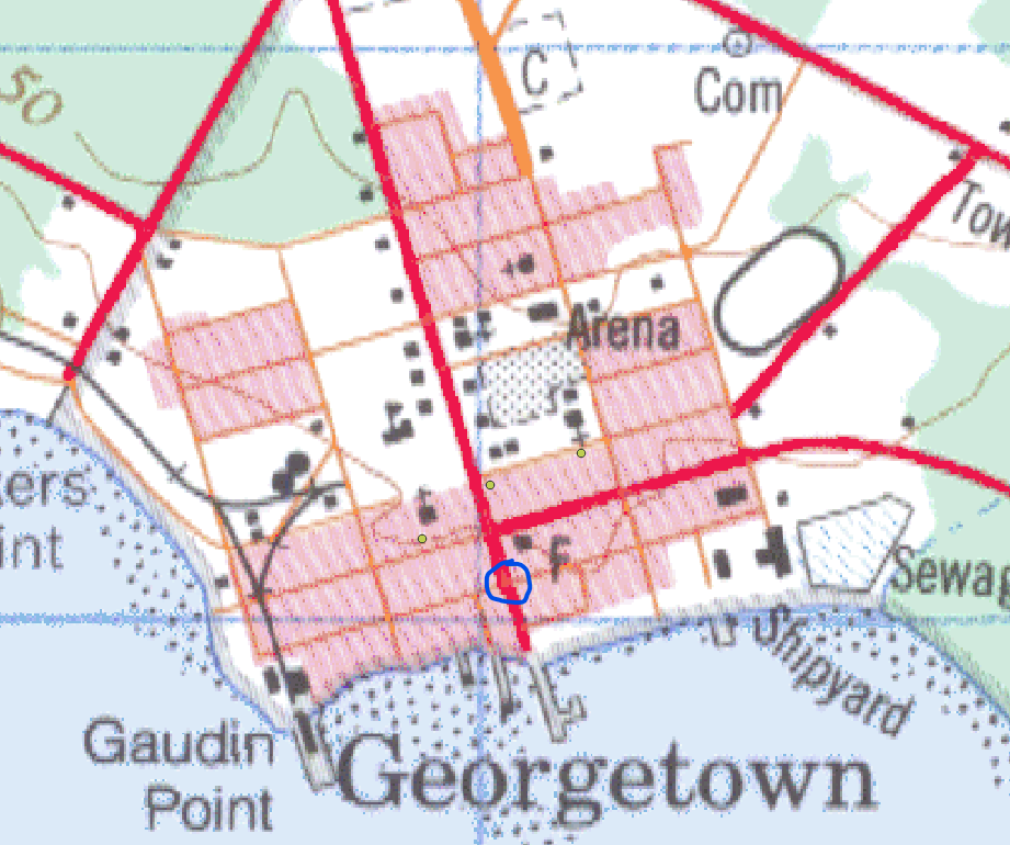
- As we did when mapping St. David’s Presbyterian Church, we will first identify the Holy Trinity Anglican Church on the NTS map. It is not named, but you will likely be able to locate it based on the screenshot below. It is represented with a cross.
- Turn off the NTS map layer, and look at the basemap. Verify the church’s location on the basemap. It is represented on the basemap with a cross.
- Click on the location of the church on the OpenStreetMap to place our point.
- In the Feature Attributes dialogue box that appears, type in the following details:
- ID: 02
- Name: Holy Trinity Anglican Church
- Click OK.
You will now see a point appear where the Holy Trinity Anglican Church is on the basemap.
Adding a Point for the King’s Playhouse
- As we did when mapping the two churches, we will first identify the King’s Playhouse on the NTS map. It is not named, but you will likely be able to locate it based on the screenshot below. There are two squares on the corner of Kent Street and Grafton Street. The King’s Playhouse is the one the furthest to the left.
- Turn off the NTS map layer, and look at the basemap. Verify the King’s Playhouse location on the basemap. You will be able to see the Playhouse’s large footprint on the corner of Kent Street and Grafton Street.
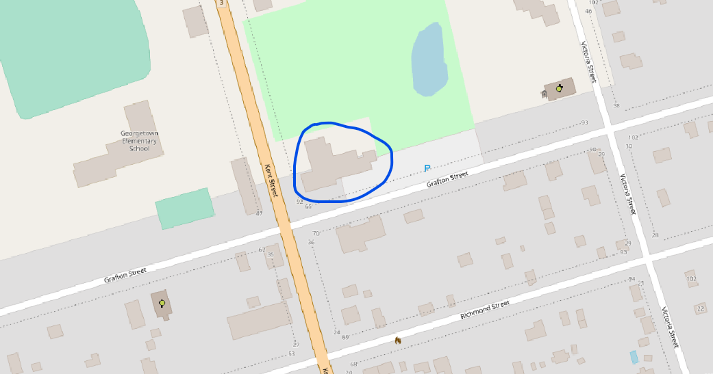
- Click on the location of the Playhouse on the OpenStreetMap to place our point.
- In the Feature Attributes dialogue box that appears, type in the following details:
- ID: 03
- Name: King’s Playhouse
- Click OK.
You will now see a point appear where the King’s Playhouse is on the basemap.
Saving the Vector Data
After we have created some vector data, we need to save it. Saving vector data is a separate process from saving the QGIS project itself. While it is also a good idea to continuously click Project > Save, after adding some vector data, we will also click the “Save Layer Edits” button.
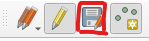
- Click the “Save Layer Edits” button.
Line
Creating a New Shapefile Layer
Once again, we will first create a new shapefile:
- Click Layer
- Hover over Create Layer
- Click New Shapefile Layer
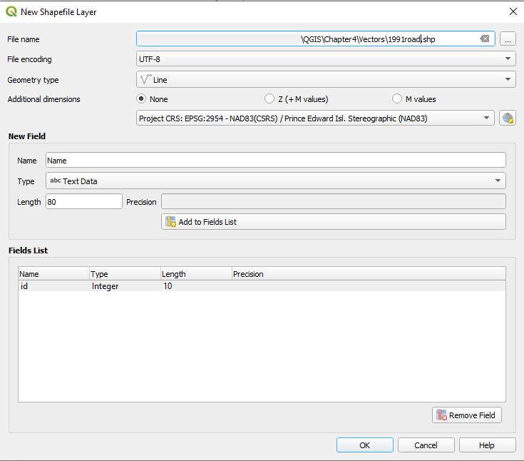
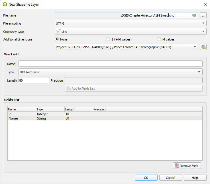
Fill out the following information in the dialogue box that appears:
File Name: …QGIS\Chapter4\Vectors\1991road.shp
- To save our shapefile in the correct location, click the ellipsis to the right of the File Name field. Navigate to QGIS\Chapter4\Vectors. Enter 1991road as the File Name, and then click Save.
File Encoding: UTF-8
Geometry Type: Line
Additional Dimensions: None
Underneath Additional Dimensions, we can also make sure the CRS is set to “Project CRS: EPSG: 2954.”
Under New Field, we can enter the following information:
- Name: Name
- Type: TextString (in some versions “Text Data”)
We can leave the other settings.
- Click Add to Fields List.
We are creating this new field so that we can keep track of the names of the places for which we are creating lines.
- Click OK
Adding a Line to the Reference Map
An Important Note about Scale
As we did when we added the points, we must consider the small scale of the NTS map when we add our line in this step. We will first identify the road for which we want to create a line on the NTS map. We will then turn off the NTS map and check the location of the same road on the basemap.
Adding the Line
- Click Toggle Editing
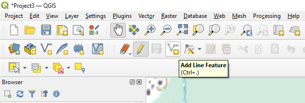
- Click Add Line Feature
Adding a Line for Kent Street
- Identify where Kent Street and North Street intersect on the NTS map.
- Identify where Kent Street and Water Street intersect on the NTS map.
- Turn off the NTS layer and look at the base map. Identify the same two points on the base map.
- Left-click once at the intersection of Kent Street and North Street.
- Move your mouse to the intersection of Kent Street and Water Street and left-click again.
- Although it is not necessary in this case, you could continue to left-click at various other points to add extra segments to your line.
- Right-click to complete the line.
- In the Feature Attributes dialogue box that appears, type in the following details:
- ID: 01
- Name: Kent Street
- Click OK.
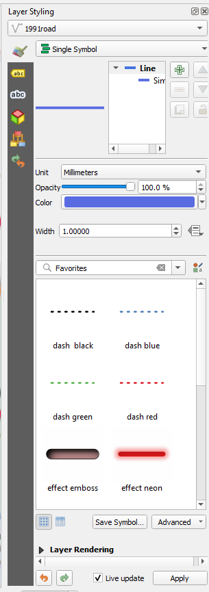
The red colour of the line we just created renders it difficult to see among the red in the NTS map.
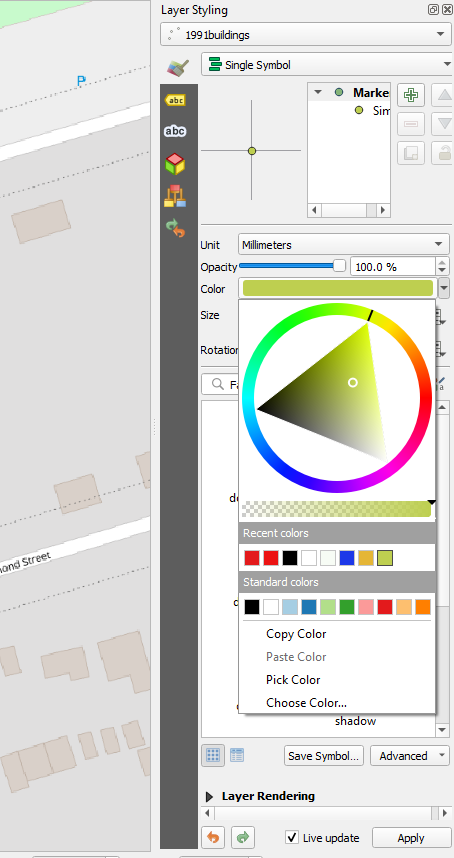
- In the Layer Styling panel to the right of your screen, click the Color dropdown menu and change the line’s colour to a purple or blue.
- Change the line’s Width to 1.0 as well.
- Click Apply
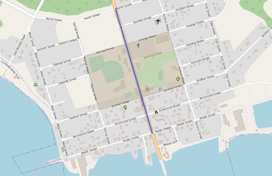
The resulting line is much easier to see:
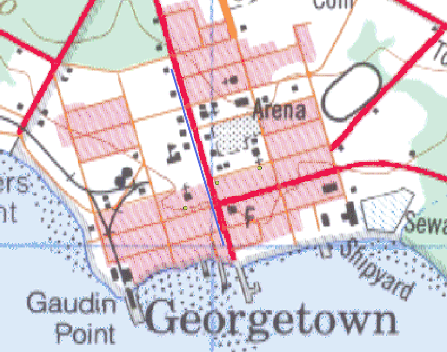
Looking at our line with the NTS layer turned on proves once again that we were able to add more accurate vector data by using the larger-scale basemap than the NTS map.
Saving the Vector Data
As always, let’s save the vector data that we just created.
- Click the “Save Layer Edits” button.
Polygon
Creating a New Shapefile
Once again, we will first create a new shapefile:
- Click Layer
- Hover over Create Layer
- Click New Shapefile Layer
Fill out the following information in the dialogue box that appears:
File Name: …QGIS\Chapter4\Vectors\1991kentsquare.shp
- To save our shapefile in the correct location, click the ellipsis to the right of the File Name field. Navigate to QGIS\Chapter4\Vectors. Enter 1991kentsquare as the File Name, and then click Save.
File Encoding: UTF-8
Geometry Type: Polygon
Additional Dimensions: None
Underneath Additional Dimensions, we can also make sure the CRS is set to “Project CRS: EPSG: 2954.”
Under New Field, we can enter the following information:
- Name: Name
- Type: TextString (in some versions “Text Data”)
We can leave the other settings.
- Click Add to Fields List.
We are creating this new field so that we can keep track of the names of the places for which we are creating polygons.
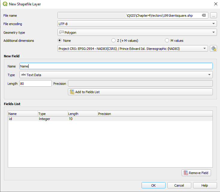
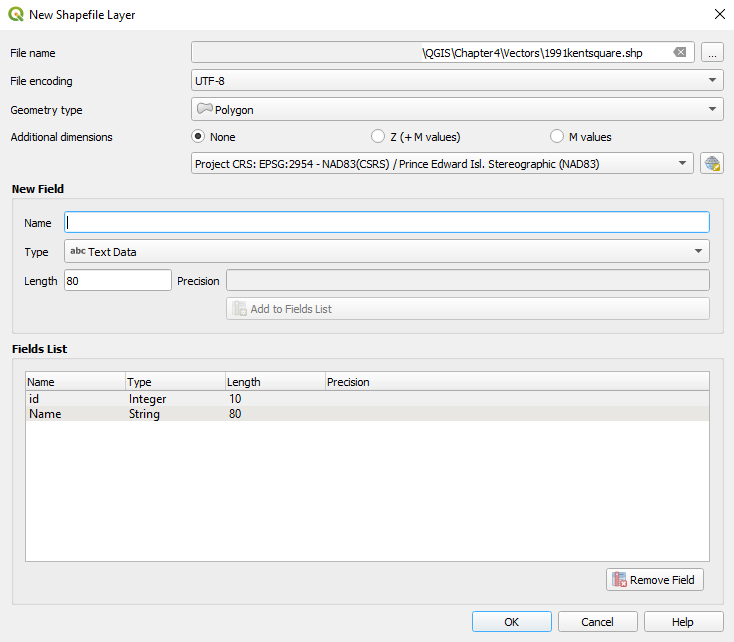
- Click OK
Adding a Polygon to the Reference Map
An Important Note about Scale
As we did when we added the points and the line, we must consider the small scale of the NTS map when we add our polygon in this step. We will first identify the area for which we want to create a polygon on the NTS map. We will then turn off the NTS map and check the location of the same area on the basemap.
Adding the Polygon
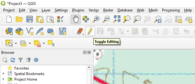
- Click Toggle Editing
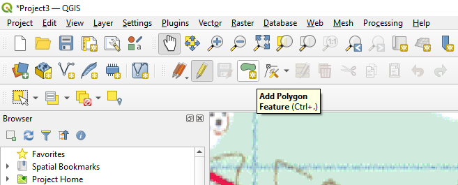
- Click Add Polygon Feature
Adding a Polygon for Kent Square
- Identify Kent Square on the NTS map.
- Turn off the NTS layer and identify Kent Square on the basemap.
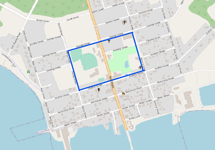 Figure 4.37
- Left-click once at the corner of George Street and Fitzroy Street.
- Move your mouse to the corner of George Street and Victoria Street and left-click again.
- Move your mouse to the corner of Victoria Street and Grafton Street and left-click again.
- Move your mouse to the corner of Grafton Street and Fitzroy Street and left-click again.
- Right-click to complete the line.
- In the Feature Attributes dialogue box that appears, type in the following details:
- ID: 01
- Name: Kent Square
- Click OK.
The resulting polygon hides part of the road and buildings layers that we previously created.
- In the Table of Contents, drag the 1991kentsquare layer beneath the 1991buildings layer.
- In the Layer Styling panel to the right of your screen, change the Opacity to 50.0%.
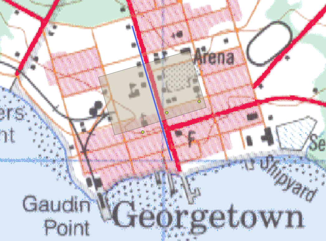
Here is the result:
If we turn on the NTS map, we can see that we placed the polygon in a much more accurate position by using the basemap.
Saving the Vector Data
As always, let’s save the vector data that we just created.
- Click the “Save Layer Edits” button.