In this step, we will download a National Topographic System (NTS) map from 1991 that has been previously georeferenced by Natural Resources Canada and shared through their Open Government portal. We will show you how to load that map into your mapping project in QGIS. The map is of a section of eastern PEI that includes the towns of Montague, Cardigan, and Georgetown. These three areas now collectively comprise the Municipality of Three Rivers.

If you do not wish to learn how to georeference your own maps at this time, you can complete this process of downloading the georeferenced topographic map and opening it in QGIS. You can use this map to continue on to Chapter 4: Digitization, where you will learn how to create your own features on the map in the form of vector data.

Loading a Base Map

Following the same instructions as Chapter 1, add your OpenStreetMap base map and set the project’s coordinate reference system (CRS) to EPSG:2954.

Downloads

• Click here to download the georeferenced copy of the 1991 NTS Georgetown map.
  • To learn more about topographic maps and the NTS map series in Canada please visit the Natural Resources Canada website.
  • The file is a zipped folder containing a GeoTIFF file.
    • The TIFF file format, which has the filename extensions .tif or .tiff, is often used for maps that are going to be georeferenced. If a file is in the GeoTIFF format, it means that the map has already been georeferenced.
    • The zipped folder also contains an xml file for one sheet in the NTS map series. The file we are interested in for this lesson is 011l02_0400_canmatrix_geo.tif. The characters “011l02” are the reference to the NTS sheet also called “Montague.”

Stream A

• Unzip the downloaded folder into your Chapter3 folder alongside your Project3 file.

Stream B

• Unzip the downloaded folder into the Rasters subfolder within your Chapter2 folder.

Adding the NTS Map

Other than the base map, the NTS map will be the first layer we add to our project.

• You can add the layer the same way you add Vectors, but instead of choosing the Add Vector Layer on the Layer Menu, choose Add Raster.
  • Or you can drag the .tif file from your computer’s File Explorer and drop it onto the map in QGIS.
• Move the new layer to the top of your table of contents by dragging the layer up and dropping it above any other layers.
• Right-click the new layer, which is called “011l02_0400_canmatrix_geo” by default, and click Rename Layer.

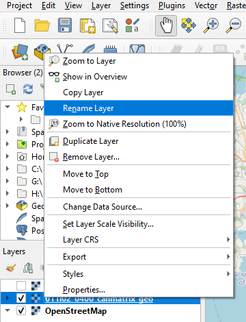
• Type in “1991 NTS Georgetown”
• Press Enter on your keyboard.

Checking the Georeferenced Map’s Accuracy

In Chapter 2: Copying a Project and Layer Styling, we learned how to adjust a layer’s transparency in order to assess its accuracy. This was useful to evaluate the precision of Holland’s map. Adjusting a raster’s transparency is also very useful to evaluate how well a georeferenced map has been aligned with our base map.

• Right-click the 1991 NTS Georgetown layer in the table of contents.
• Click Properties
• Click Transparency
• Change the Global Opacity to 30%.

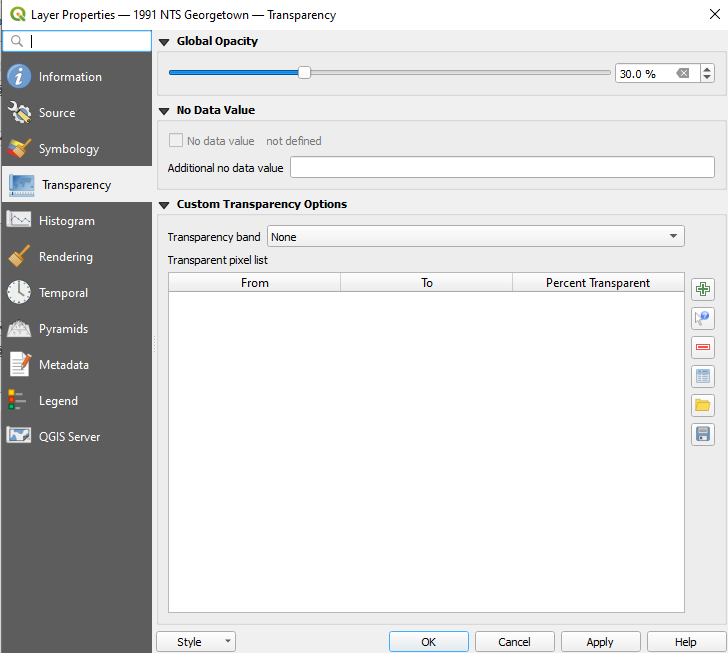
• Click OK.
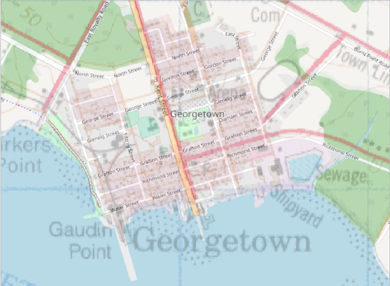
• Zoom into the Georgetown area.
• Compare the streets in the NTS map with those in the underlying OpenStreetMaps base map. How well do they align?

In the screenshot below, we can see that there is a slight misalignment between the streets in the NTS map and those on the base map. For example, on the NTS map, Kent Street is located slightly east and Richmond Street is slightly north of their respective locations on the base map. But, overall, the two maps align well. So, we know that the georeferencing is fairly accurate.

Continue to Georeferencing in Stream B or Skip to Chapter 4

If you are only interested in learning how to add a georeferenced map to your GIS at the moment, you can now skip ahead to Chapter 4: Digitization.

Why Is It Helpful to Learn How to Georeference?

You may choose to skip the process of learning how to georeference because you already have access to georeferenced maps. Indeed, many of these can be found online. However, it is very beneficial to learn how to georeference, as it opens up the opportunity to work with many more maps. Of the digital maps out there, the vast majority have not yet been georeferenced. When you learn how to georeference, you will not be constrained to working with the limited number of pre-georeferenced maps. You will be free to take any digital map and georeference it yourself.

As a case in point, consider the georeferenced NTS map provided above. If we limited ourselves to this map, we would have to settle for its scale, which is a little too zoomed out for a detailed study of Georgetown. We would also have to settle for the map’s time point, 1991, which is not very historical. But, once we know how to georeference, we can take a digitized map from the 1880 Meacham’s Atlas that shows Georgetown at a much closer scale and at a much older time point. Such a map is much more useful to us in our study of how Georgetown’s prosperity from this time withered away.