Chapter 5: Creating an Exportable Map in QGIS
Becoming a Cartographer: Creating a Layout
If we wish to create a more sophisticated output of our map, one that includes items such as a legend and north arrow, we can create a layout.
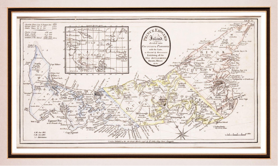
We create layouts in the Print Layout window. This interface is different than the one that we have used thus far for mapping, which is called the Main Canvas. In the Print Layout window, we have all the options we need to design our map output. As we do so, we are engaging in the practice of cartography, which introduces artistic expression into the scientific practice of mapmaking. In the past, cartographers spent a great deal of time and effort to create their maps by hand. Let’s remember the map of Prince Edward Island that we saw in Chapter 1, a beautiful work of art created by Captain Holland and revised by successive generations of mapmakers. The 1798 version that we used was produced—painstakingly, no doubt—by the mapmaker H. Ashby in London, United Kingdom.
In this part of the chapter, we will use modern-day methods continue in this age-old tradition of designing an accurate and appealing map.
As cartographers, we are telling a story with our map. We have a choice in how we wish to present spatial data in order to tell this story. Our decisions shape how an audience interprets our map. As when writing a story, it is advisable to consider your purpose and audience when telling a story through spatial means.
Opening the Print Layout Window
To open the Print Layout window:
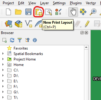
- While in the Main Canvas, click the New Print Layout button located at the top-left of the main QGIS window.
After clicking New Print Layout, the following window will pop up:
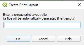
- Type in “Chapter 5 Layout”
- Click OK.
A new window will pop up containing the Print Layout interface.
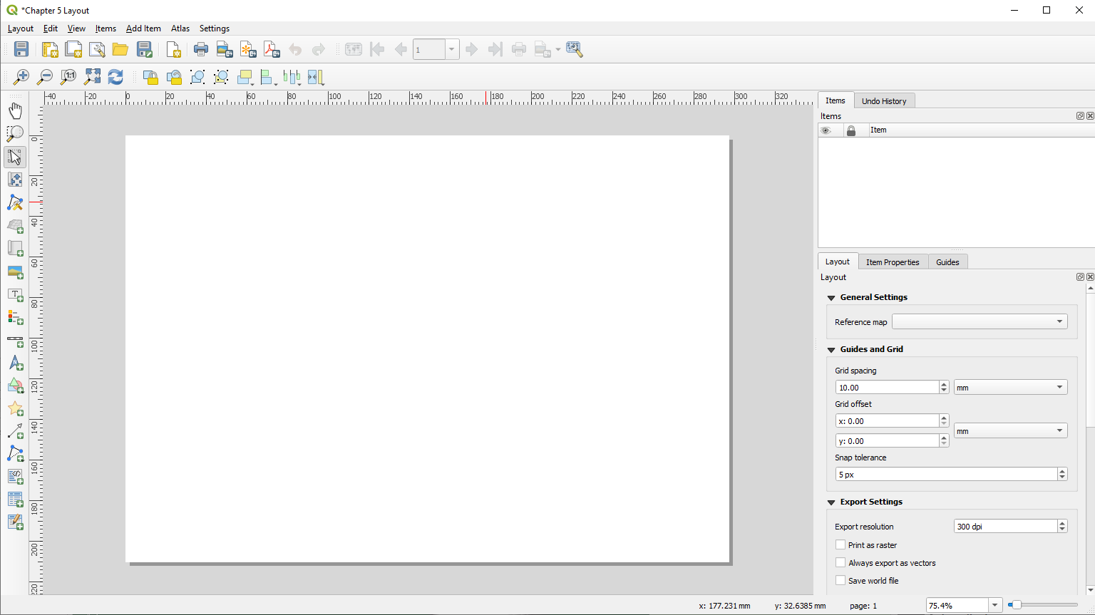
You will now have two QGIS windows open: one for the Main Canvas and one for the Print Layout.
The layout will initially be a blank white page. In the following steps, we will add our spatial data and some metadata.
Setting the Page Size
When we create layouts, the goal is often eventually to print them. We may want to specify which size of paper onto which we will eventually print our layout. To set the page size:
- Right-click anywhere in the blank white space of the layout page.
- Click Page Properties
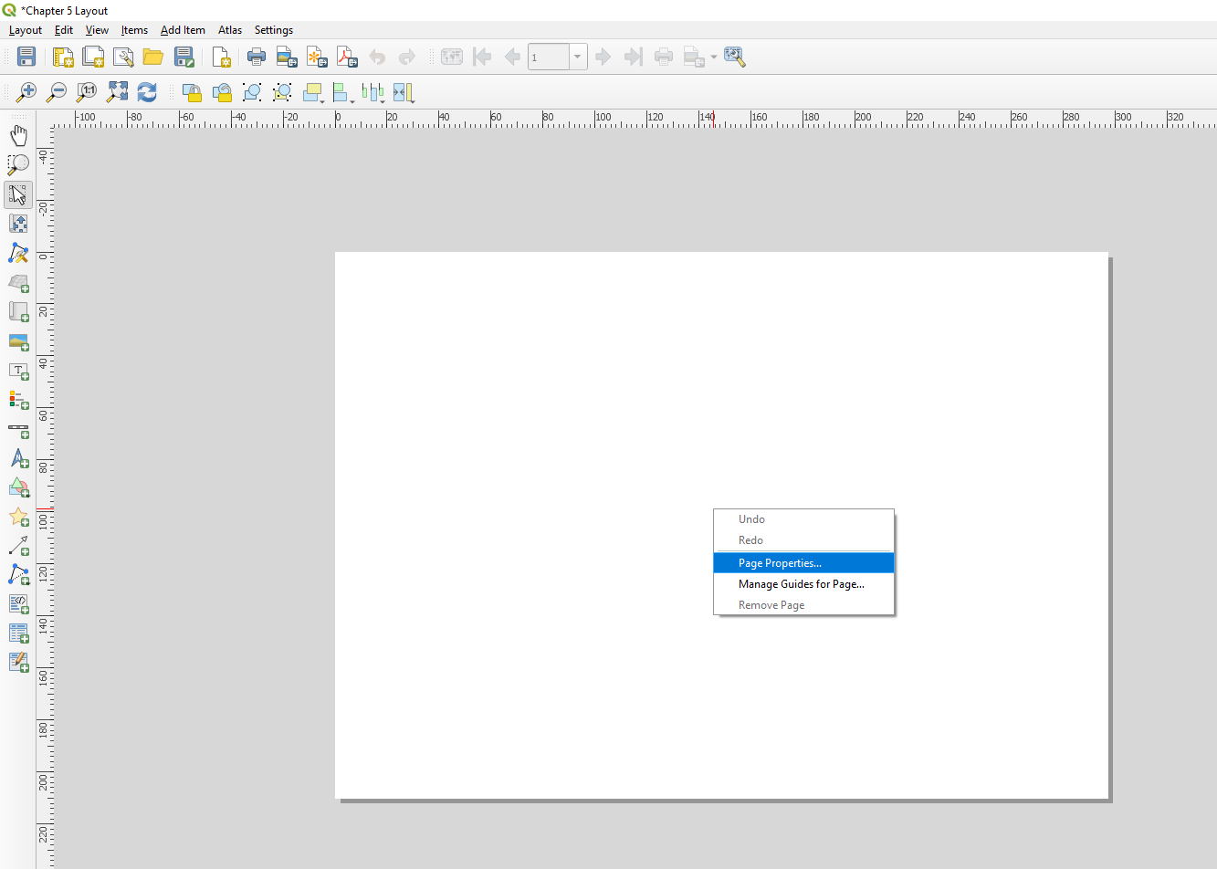
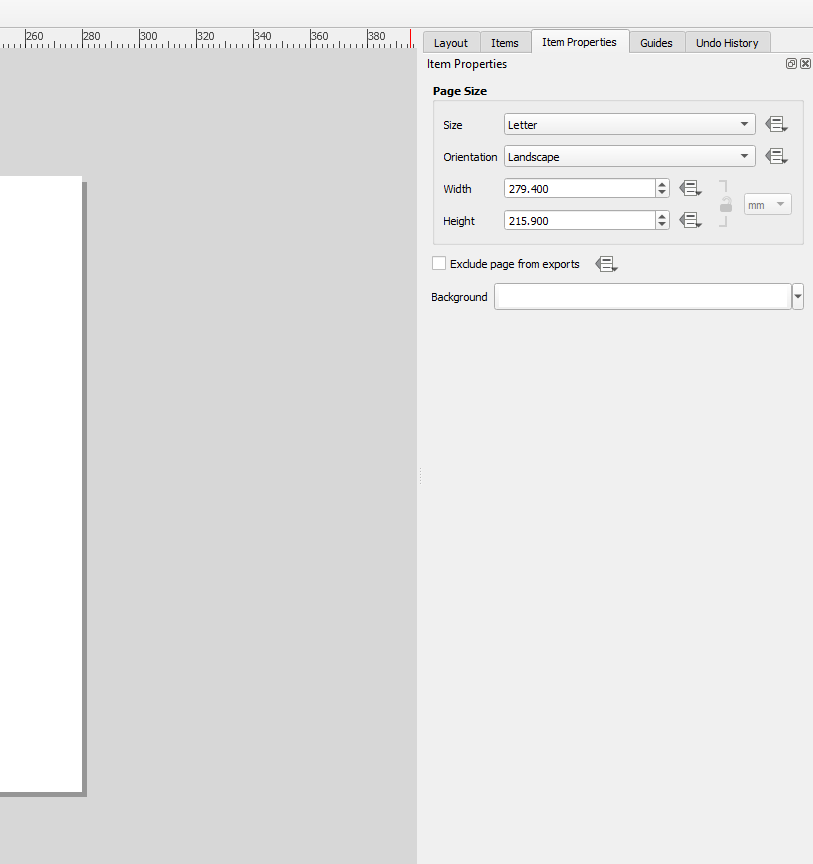
- In the Item Properties tab to the right, change the size to one you prefer. We have chosen Letter.
- You can also change the orientation to portrait if you would like, but the rest of this chapter will be done in a landscape orientation.
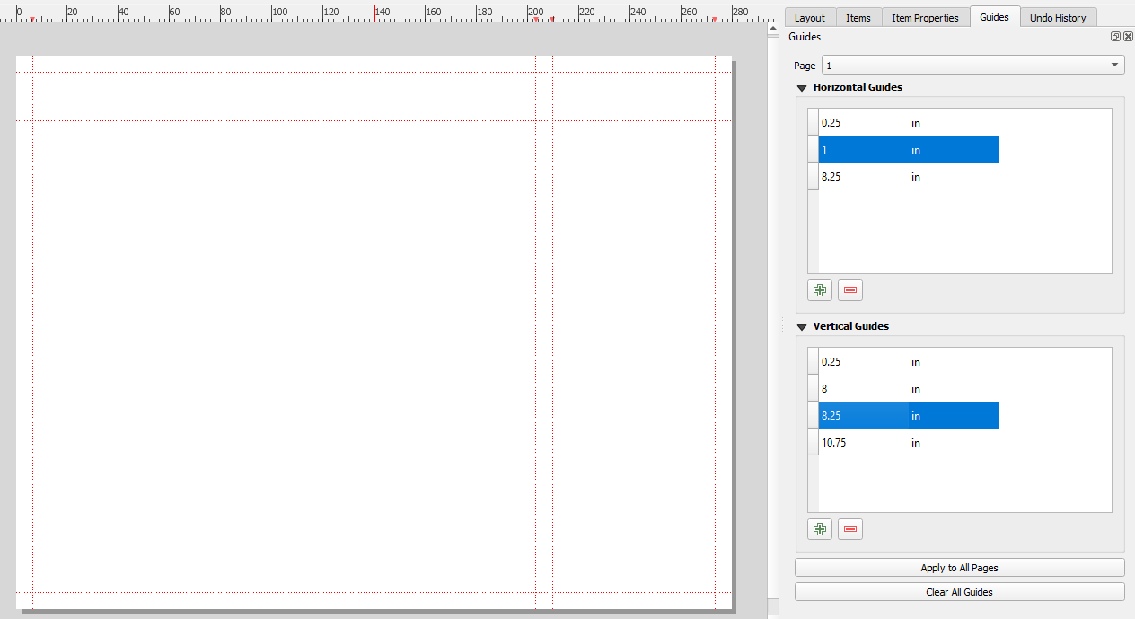
Adding Guidelines
We will create some guidelines to help us place our map, legend, and other items precisely on the map layout page. These guidelines will not appear in the file that we output at the end.
We will first add some guidelines to demarcate the outer limits of our page.
- Right-click anywhere in the blank white space of the Print Layout page.
- Click Manage Guides for Page
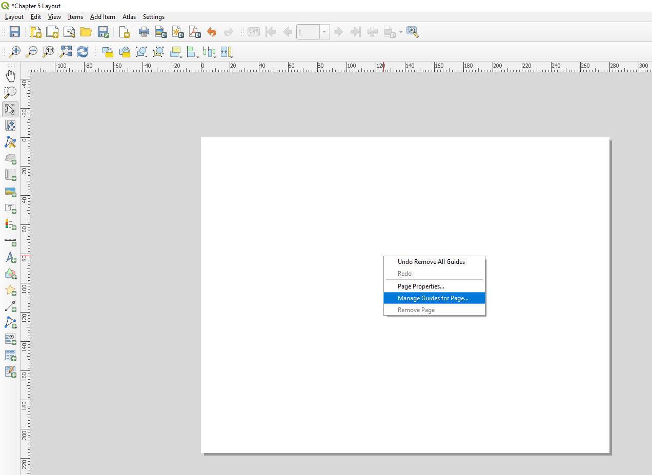
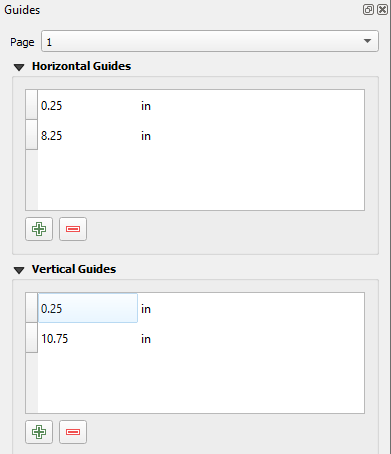
- In the Guides tab to the right, click the green plus button to add a horizontal guide at 0.25 inches.
- Add another horizontal guide at 8.25 inches.
- Enter two vertical guides: one at 0.25 inches and one at 10.75 inches.
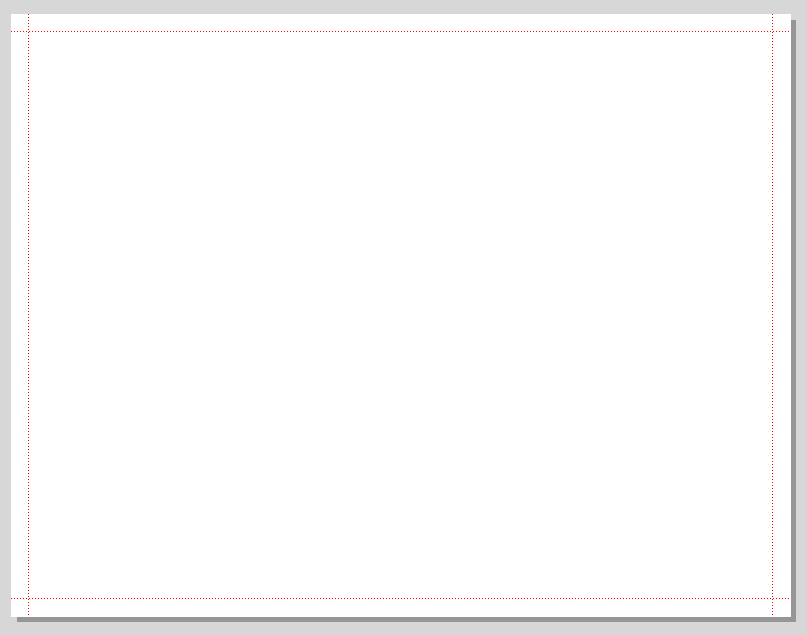
We will now add guides to divide our page into sections. We will add our spatial data and metadata into these sections.
Let’s create an area into which we can type the title of our map.
- Add a horizontal guide at 1 inch from the top of the page.
INSERT PICTURE HERE**********************************
We can also create areas on the right-hand side and bottom of the map where we can place the rest of our metadata.
- Add two vertical guides: one set at 8 inches and one set at 8.25 inches.
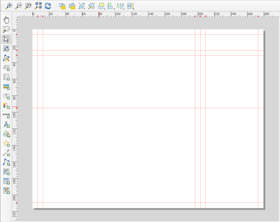
Finally, we will add a few more guidelines that will demarcate the position of the inset map that we will add in subsequent steps.
- Add one horizontal guide at 1.25 inches and one at 3.75 inches.
- Add one vertical guide at 0.5 inches and one at 7.75 inches.
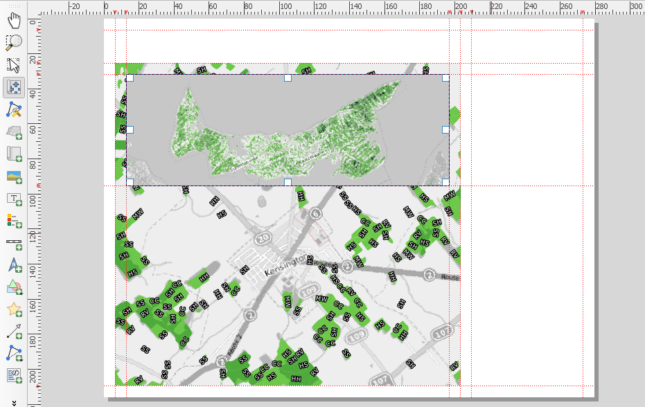
Your layout page will now look like this:
Adding Maps to the Layout
We can use the guidelines we just created as we add our map and metadata to our print layout page.
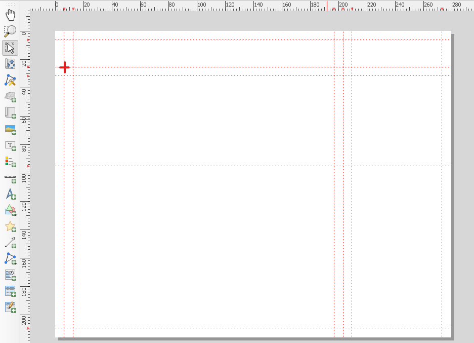
Adding the Main Map Frame
When we add an image of our map to the print layout page, it is called a map frame. To add the main map frame to our layout,
- In the toolbar on the left of the screen, click Add Map. (This tool allows us to add map frames.)
- The layers that we will add when we click this button is the ones that we currently see in the Main Canvas of QGIS. Make sure you go to the Main Canvas and turn on the layers that you would like to add to the layout before you click the Add Map button. In this case, we turned on the 1935 inventory region filtered and graduated layer and the OSM Grayscale layer.
INSERT PICTURE HERE**********************************
- With your cursor as a crosshairs, left-click and hold on the top-left corner of the central box we created with our guidelines.
- Drag to the bottom-right corner of the central box and let go of the click there.
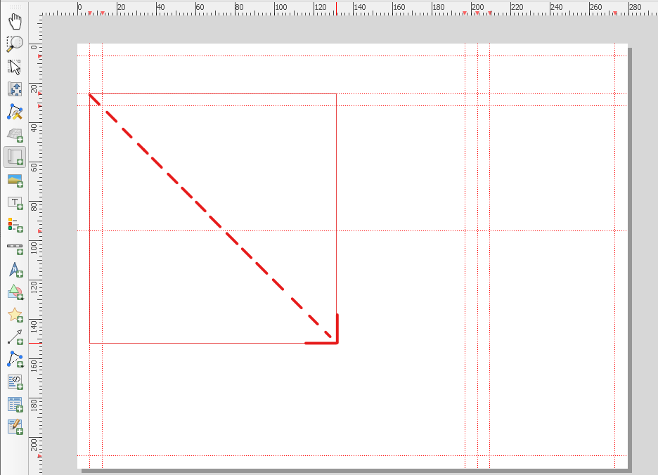
The map that you can see in the main mapping view will render.
Pan to Kensington
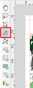
- In the toolbar on the left-hand side of the layout window, click the button called Select/Move an Item
INSERT PICTURE HERE**********************************
- Click to select the main map frame.
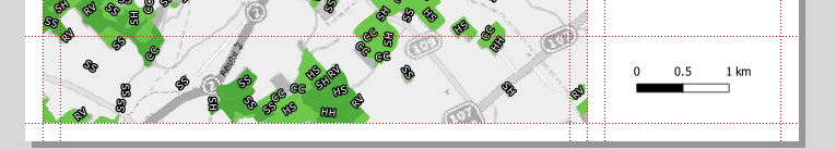
- In the Item Properties menu to the right, under Main Properties, change the scale to 30000.
- Change the map rotation to -25.00 degrees.
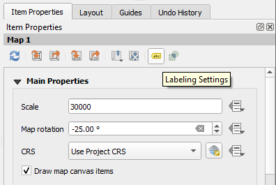
- Still in Item Properties, under Extents, change the extent values to the following:
- X min: 348336.227
- Y min: 707573.371
- X max: 354241.728
- Y max: 713097.871
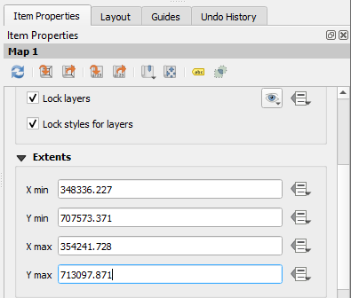
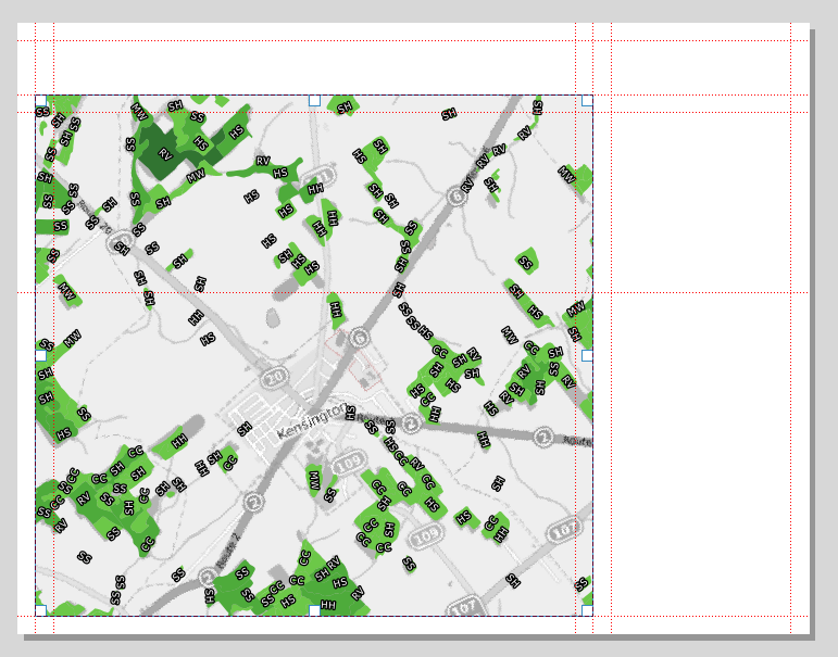
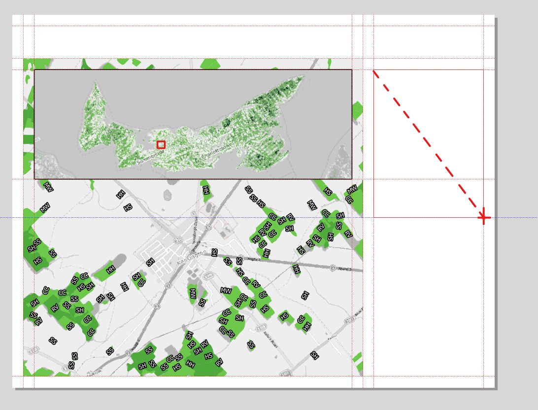
After entering the above extents, this is what we see:
Locking the Appearance of the Main Map Frame
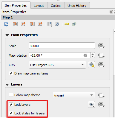
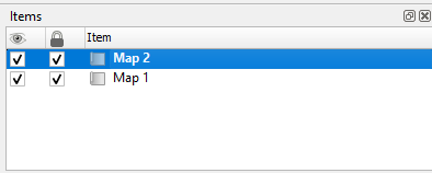
Below, we will add an inset map and make other changes to our layout. As it stands right now, the main map frame in our layout is dynamically linked to the map in the Main Canvas. So, when we make changes to the latter, the map frame in our layout will refresh to match. (This refreshing will happen automatically or if we click the Refresh View button.) We want to prevent the main map frame from refreshing as we add our inset map. To do so, we will use a setting called Lock Layers.
- Click on Map 1 (i.e., the main map frame) to select it in the Items list.
- Under Layers, click Lock layers and Lock styles for layers.
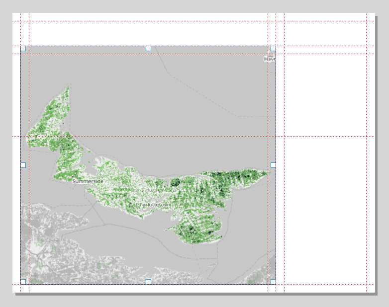
Adding an Inset Map
We will now add an inset map in order to give the audience some context as to where Kensington is in relation to the surrounding parts of PEI.
- In the Main Canvas, turn off the PEI placenames layer so that the only layers visible are the 1935 inventory region filtered and graduated layer and the OSM Grayscale layer.
- In the Print Layout window, click Add Map and click and drag to insert it into the 2.5-inch by 7.25-inch area that we created with our guides.
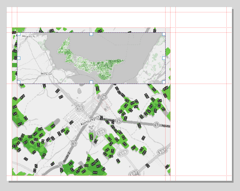
Panning the Inset Map
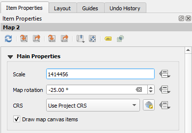
In the Items pane, click to select Map 2 (i.e., the inset map).
In the Item Properties pane, under Main Properties, set the Scale to 1414456 and the Map rotation to -25.00 degrees.
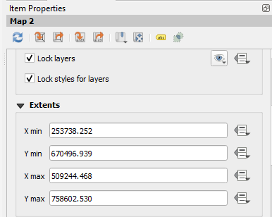
- Under Extents, enter the following:
- X min: 253738.252
- Y min: 670496.939
- X max: 509244.468
- Y max: 758602.530
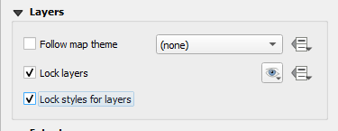
- With Map 2 selected in the Items pane, click Lock layers and Lock styles for layers.
This is what our layout looks like so far:
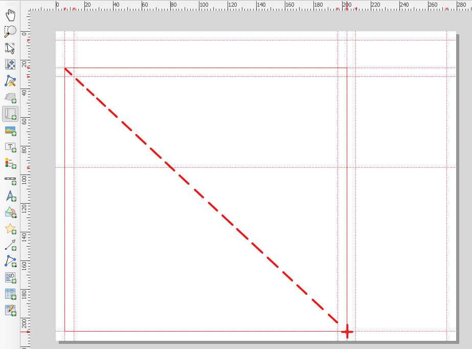
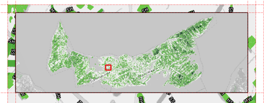
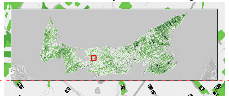
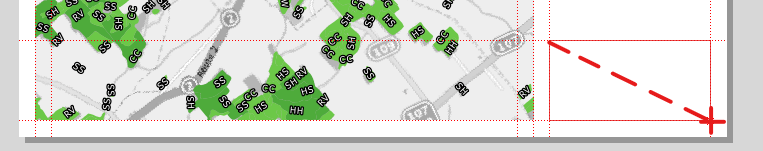
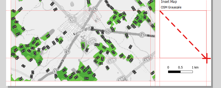
Adding an Extent Indicator
The inset map’s purpose is to show the audience the geographic context of Kensington, the place shown in our main map frame. However, it may remain unclear as to where Kensington lies within this inset map. For this, we can add an extent indicator using the Overview function in QGIS.
- With Map 2 selected in the Items list, in the Item Properties tab, under Overviews, click the green plus button to add an overview.
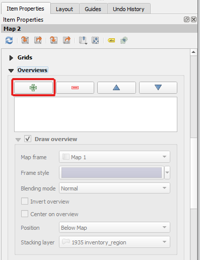
An overview called Overview 1 will appear in beneath the green plus button.
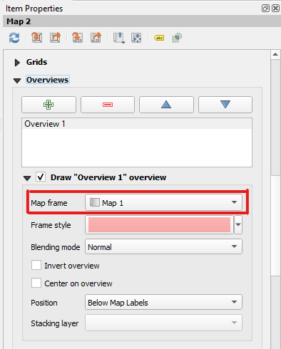
- In the dropdown menu next to Map Frame, select Map 1.
- This is the map frame over the top of which QGIS will place our extent indicator.
A semi-transparent red extent indicator will appear over the top of the inset map. It covers the area that we see in the main map frame. We will change this appearance to a solid red outline so that it is more visible.
- Click the dropdown arrow next to Frame style.
- Click Configure Symbol.
- Click Simple Fill to select it.
- Click the dropdown arrow next to Fill colour
- Under Standard Colours, click red.
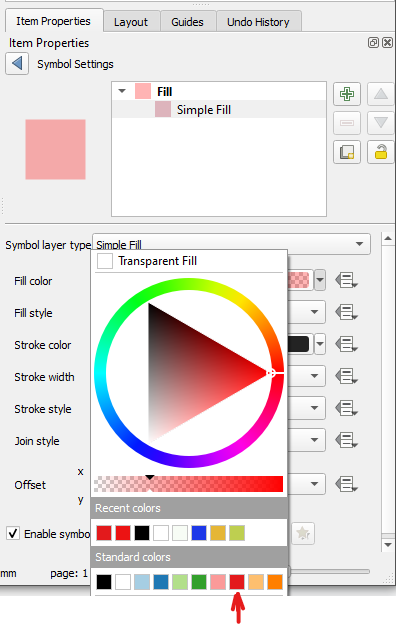
- Click the dropdown arrow next to Fill Style
- Choose No Brush
- Click the dropdown arrow next to Stroke colour
- Under Standard Colours, click red.
- Change the Stroke Width to 1.00 millimetre.
- Change the Stroke style to Solid Line.
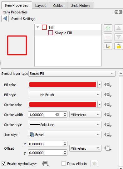
Here is the result:
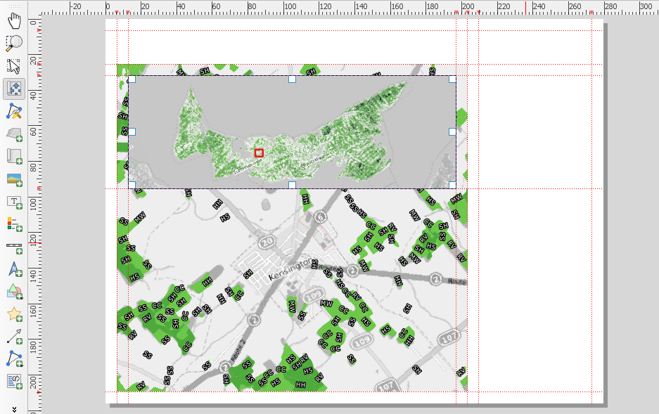
Adding a Border around the Inset Map
A border around our inset map may help an audience to see that it is distinct from our main map.
- Use the Select/Move Item tool to select the inset map.
- In the Item Properties tab, check the box next to the word Frame.
- Under Frame, leave the colour as black, set the thickness to 0.50 mm, and set the Join Style to Round.
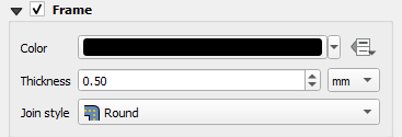
The result may be hard to see with our guidelines on, but it is there, and it will become more visible once we export the layout as an image or PDF later in the chapter.
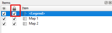
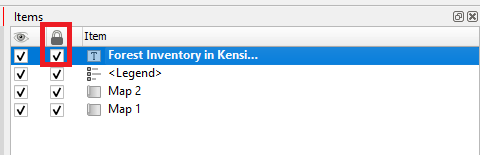
Locking the Positioning of the Layers
We have already locked the appearances of the main map frame and the inset map. Now, we will lock the locations of these map frames on the page. This ensures that we cannot accidentally alter the size or location of the map frames.
- In the Items pane, under the symbol of the padlock, check the box for Map 1 and Map 2.
Now, if we try to use the Select/Move Item tool to select either the main map frame or the inset map frame, we cannot.
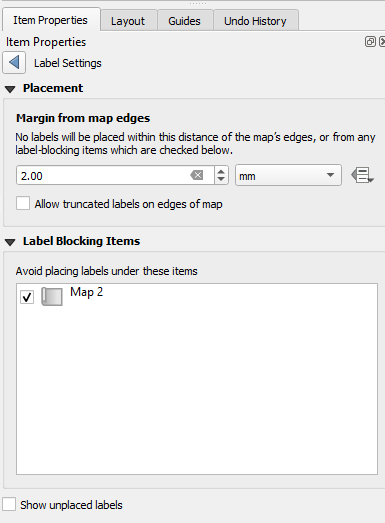
Label Settings
Before we move on, let’s adjust the label settings so that labels are not drawn too close to the edge of the map frame. We can also change the settings so that the labels on the 1935 forestry inventory map located underneath the inset map are not drawn.
- Click Map 1 in the Items list.
- In the Item Properties tab, click the Labelling Settings button.
- Under Placement, change the Margin from Map Edges value to 2.00 millimetres.
- Under Label Blocking Items, select Map 2.
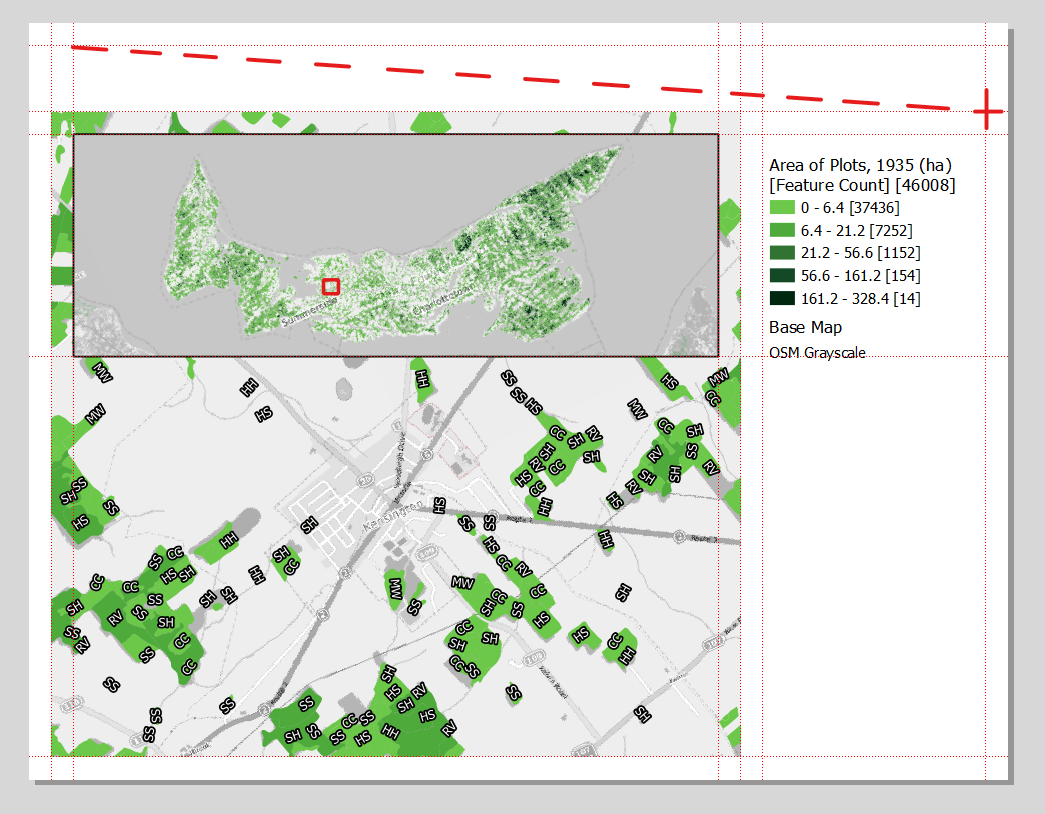
We can now see how QGIS does not draw labels on the main map that would be too close to the inset map:
Adding Metadata to Our Map
We will now add some metadata around our map frames to help an audience understand our maps.
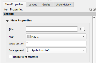
Adding a Legend
We can add a legend to help users understand the colours of our choropleth map.
- Click Add Legend
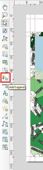
- Place the legend in the space created by the guidelines to the right, using the same click and drag method that we used to add the map frames. When you drag to point that is halfway down the page, a temporary, blue guide will appear. Let go of your click at this point.
We will now start to edit our legend’s information.
- Under Main Properties, leave the Title field empty.
- Make sure Map 1 is selected in the Map field.
- In the field called “Wrap text on,” enter an asterisk (i.e, *).
- This prepares us to be able to wrap text in our legend in subsequent steps.
- Leave the Arrangement at Symbols on Left
- Uncheck Resize to Fit Contents.
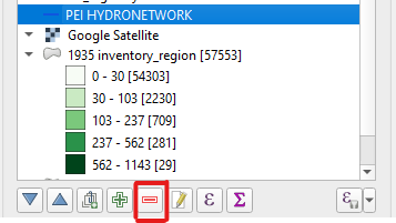
- Under Legend Items, uncheck Auto Update.
- This will allow us to change the legend items manually.
- Select any layers other than the 1935 inventory region filtered and graduated layer and the OSM Grayscale layer.
- With these unwanted legend items selected, click the red minus button to delete them.
With all of the unwanted layers deleted from the legend, we can now rename the layers that we want to keep.
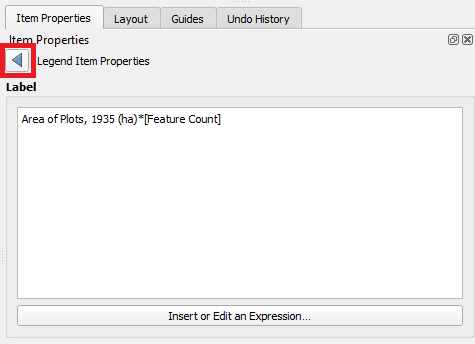
- Click to select the 1935 inventory_region filtered and graduated layer.
- Click the button called Edit selected item properties.
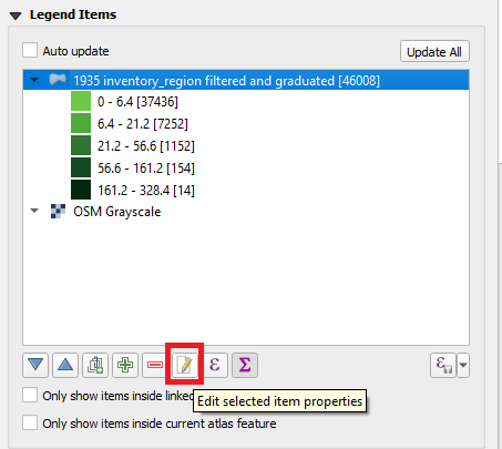
- Type in “Area of Plots, 1935 (ha)*[Feature Count]”
![Figure 5.54. This shows under Item Properties, Label is written “Area of Plots, 1935 (ha)*[Feature Count]”. In the image it is shown with a red box around it.](http://pressbooks.library.upei.ca/geospatialhumanities/wp-content/uploads/sites/53/2022/03/image106.png)
Click the back button to return to the rest of the settings.
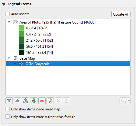
Next, we are going to group and order our legend items.
- Click the Add Group button.
- Rename this group to “Base Map.”
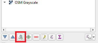
- Click and hold on the OSM Grayscale layer, drag it over the top of the Base Map group, and release.

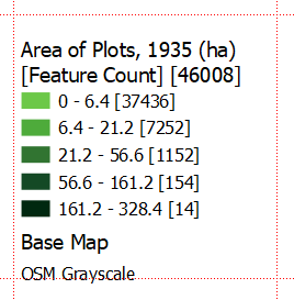
We will now change the appearance of the items in the legend in the Print Layout page.
- Right-click the legend item called “Area of Plots (ha), 1935*[Feature Count]”
- Click Group
![Figure 5.59. In the Legend Items “Area of Plots (ha), 1935*[Feature Count]” is selected and the option Group has a check mark beside it.](http://pressbooks.library.upei.ca/geospatialhumanities/wp-content/uploads/sites/53/2022/03/image116.png)
- Right-click the Base Map group and make sure it is a Group.
- Right-click the OSM Grayscale layer and make sure it is a Subgroup.
- Arrange the layers so that the “Area of Plots (ha), 1935*[Feature Count]” layer is at the top and the Base Map group is at the bottom.
![Figure 5.60. In the Legend Items “Area of Plots (ha), 1935*[Feature Count]” layer is at the top and the Base Map group is at the bottom.](http://pressbooks.library.upei.ca/geospatialhumanities/wp-content/uploads/sites/53/2022/03/image118.png)
Here is the result on the Print Layout page itself:
- Before moving on, lock the legend in the Items list.
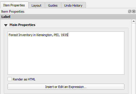
Adding a Title
We can now move on and add a title to our map.
Click Add Label.
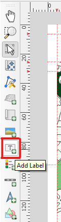
- Click and drag to insert the textbox across the top of our main map frame, nestling it within our guidelines.
- Under Main Properties, type in “Forest Inventory in Kensington, PEI, 1935”
- Under Appearance, click the dropdown arrow next to Font and change the font size to 40.
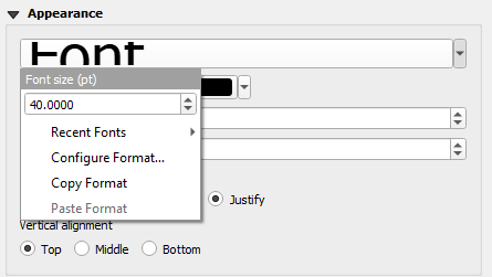
- Change the Horizontal Alignment to Left.
- Change the Vertical Alignment to Middle.
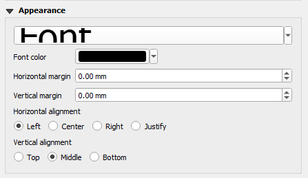
Here is the result:
Before moving on, lock the title in the Items list.
Adding a Scale Bar
Adding a scale bar will help our audience to understand the distances on our map in relation to the real world.
- In the Guides tab, add a horizontal guide at the 7-inch mark.
- Click the Add Scale Bar button.
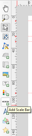
- Draw a scale bar between the 8.25-inch mark and the 7-inch mark.
- Use the Select/Move Item tool to select the scale bar.
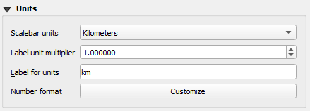
- In the Item Properties tab, under Units, change the Scalebar units to Kilometres.
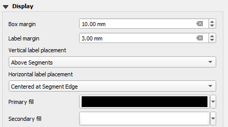
- Under Display, change the Box margin to 10.00 mm.
- This will have the effect of centring our scale bar.
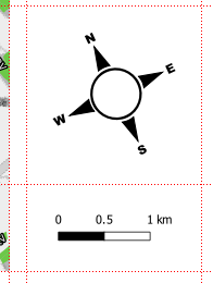
Here is the result:
Adding a North Arrow
A north arrow can help someone looking at our map to understand the orientation of our map frame.
To add a north arrow,
- Add a horizontal guide at the 4.45-inch mark.
- Click the Add North Arrow button.
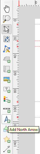
Draw a north arrow between the 4.45-inch mark and the 7-inch mark.
We can now change the appearance of our north arrow if we wish.
- Use the Select/Move Item button to select the North Arrow.
- In the Item Properties tab, make sure the SVG Image radio button is selected.
- In the list of SVG Groups, under “App Symbols,” click “arrows.”
- Choose the four-headed compass rose that features the letters N, E, S, and W.
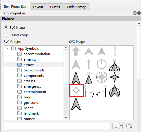
Under SVG Parameters, change the Fill colour to black.
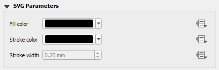
We can now see the compass rose on our layout page:
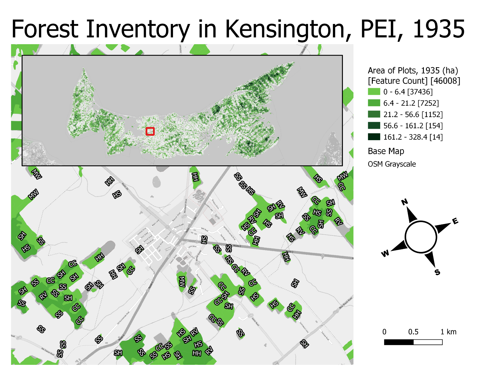
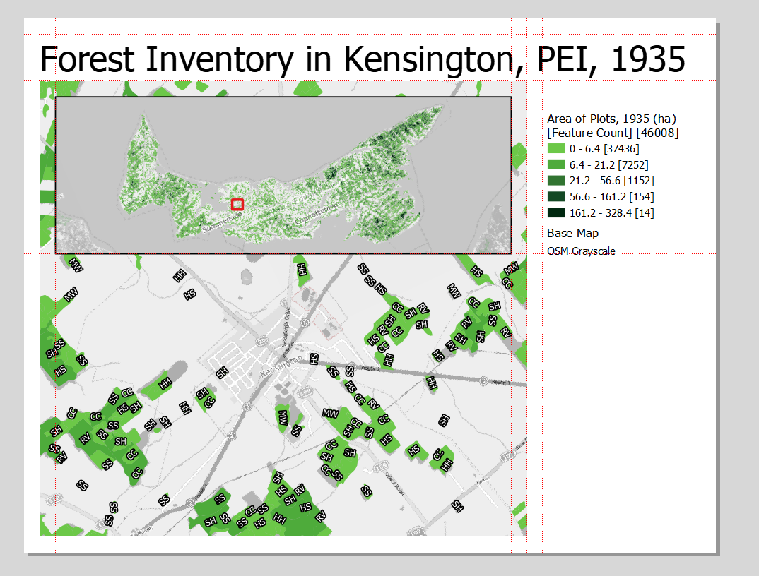
Here is the final result of our layout in the Print Layout window:
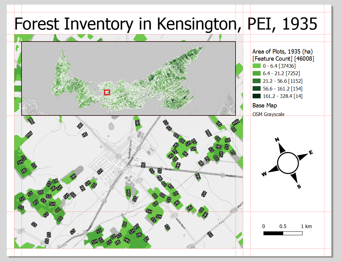
Our layout is now complete and ready to be exported.
Exporting Our Layout
We have a few options for exporting our layout.
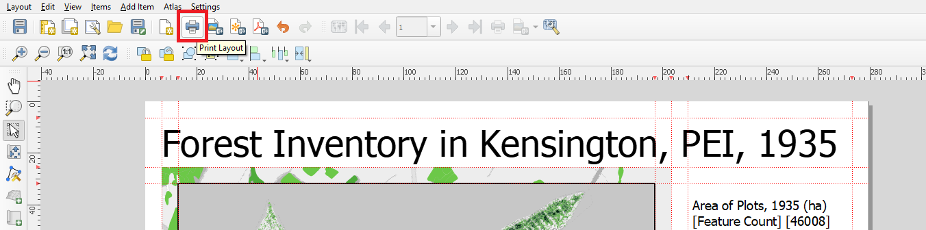
We can print our layout directly from the Print Layout window.
If you wish to print your layout, click the Print Layout button.
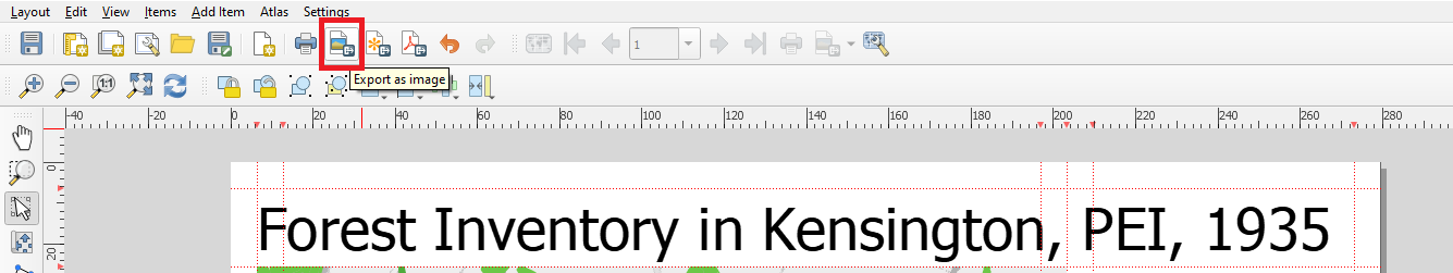
Saving as an Image
We also have an option to save our layout as an image file. We could print this file later.
If you wish to save your layout as an image file, click the Export as Image button.
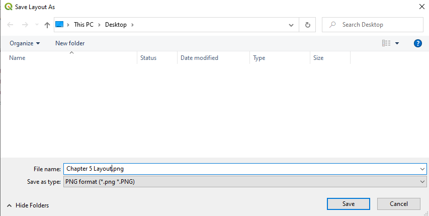
A window will then pop up and ask you where you would like to save your file.
Navigate to an appropriate location, provide a file name, and click save.
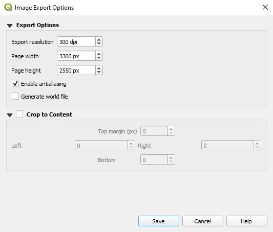
Another window will pop up called Image Export Options.
- You can leave the settings at their defaults and click Save.
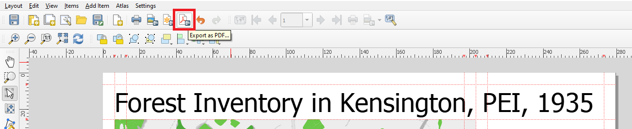
Saving as a PDF
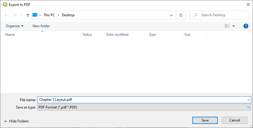
We can also export our layout as a PDF.
If you wish to export your layout as a PDF, click the Export as PDF button.
A window will then pop up and ask you where you would like to save your file.
- Navigate to an appropriate location, provide a file name, and click save.
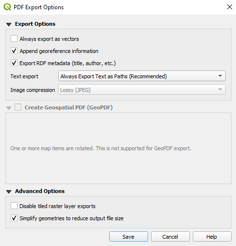
A window will pop up asking you to specify the settings for your PDF.
- You can leave the settings at their defaults and click Save.
The Final Result
Here is the final result of our print layout exported as an image file.