Spreadsheet Basics in Excel

Remember that the main strength of spreadsheet programs is to manipulate numbers. If you know how to do something in one program, you can be pretty sure that the same options are available in the other program, but it may not be called the same thing. So we’ll run through some of the main options Excel to give you some idea of how to use some of these options.

Data manipulations

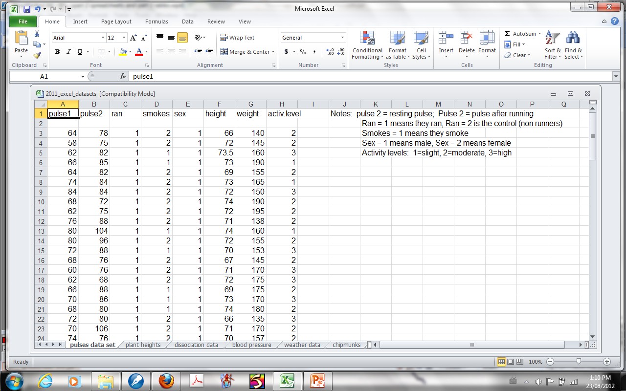
Most of the examples in this guide refer to a dataset on your Moodle site called the “pulses” dataset. It consists of sample data from a study where a researcher had his class take their pulse rate to give a “baseline” value, then part of the class ran in place for one minute, and the class members took their pulse rates again. After the experiment, the researcher asked the students what their normal activity level was, whether they smoked, what sex they were, and what their height and weight were. This gives us a useful dataset to evaluate a number of different techniques, and if you want, you can try out these methods to make sure you understand how to do them.

If you open your “pulses” dataset, your excel spreadsheet should look like the one given below.

Sorting Data

The ability to sort the data is one of the most useful data manipulations available with a spreadsheet.

For this example, we’ll use the “pulses dataset” available on your disk.

Method:

• Open the pulses dataset. Depending on how your data are set up, you may need to use the mouse to select the data you would like to sort (if you don’t highlight the data first, the program will highlight all of your data, including headers and any notes you might have).
  • Important: be sure all data columns in your dataset are highlighted or selected. Otherwise you will only sort the selected columns, and your other data may get out of synchrony with the new sorted data.

• Click on the “Data” tab at the top, and then choose the “Sort” icon. Click on it to open the sort window
• Click on the small arrow beside “sort by” and a drop down menu showing your column titles (A, B, C….). – Choose the Column that you wish to sort by (for example, if we wished to sort by whether they smoked or not, we would choose column D). If you check the box for “my data has headers” then you will see the heading names instead of the column letter

Notice at the top left of the Sort window… there is a box to “add level”. You would use this if you wanted to be able to sort by more than one category. For example, if I wanted to sort so the runners came first, and then the non-runners, but I also wanted to sort the smokers within each running group, I’d do it by specifying a second level. First choose column C, then click on Add Level. This adds a second level for your sorting, and you can specify column D. Finally, for each level, choose whether you want ascending (lowest to highest) or descending numbers.

• Click ok. Your data should now be sorted.

Arithmetic Functions

A major strength of spreadsheets is the ability to do repetitive arithmetic functions easily.

How to access the arithmetic functions in Excel:

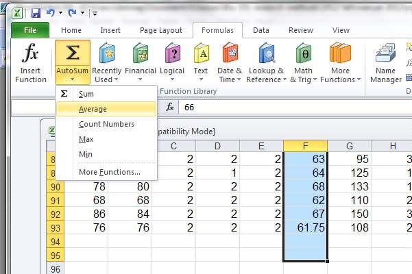
• Click on the Formulas tab, and look for the 3 symbol in the Excel property bar. Notice the small arrow beneath the 3 key… click on that to get the most common arithmetic functions, then choose “more functions” to get into any additional ones you may need.
  • Hint: if you want to sum other columns now, you can just copy the arithmetic function (=SUM…) from your first column and paste it into the same cell for other columns. The computer will automatically adjust the column letters, so that you get the sum of the appropriate column.

Sums

• To sum all the values in a column or row, simply place your cursor in a blank space at the end of a row or column and click on the auto-sum key. Then hit the Enter key, to get your value.
• To sum the numbers in only part of the column or row, highlight the numbers you want summed before clicking on the sum key.

Averages

• Click on the small arrow below the 3 key on the property bar, and choose “average” from the drop-down menu.
  • Hint…. you can do this calculation for multiple columns, by copying and pasting the formula into an adjoining cell.
    To obtain an average for an entire column or row, simply place your cursor on a blank cell at the end of the row or column, then click on average from the autosum drop down menu.
• To obtain an average for a subset of values, highlight the values before clicking on “average”.

Other statistical functions

• First place your cursor on an empty cell at the bottom of the column or to the right of the row you want analysed.
• Now access the other functions by clicking on the small arrow below the 3 icon on the functions tab of the property bar, and clicking on “more functions” from the drop-down menu to get the Insert Function box
• You can type in a brief description of what you would like to do (e.g. “Find the median”), or you can select a function category.
  • If you click on the “select a category” window, you’ll see a listing of the different categories available
• For the statistical functions, click on “statistical”, and choose from the listing.
  • e.g. standard deviation of the mean for Column F of our pulses dataset
  • click on an empty cell and choose STDEV.S from the statistical list. In the “function arguments” dialogue box, choose the data you want to analyse.
  • If you don’t do anything else, it will calculate the value for all the numbers in the column.
• For a subset of the column (or a different column), either type in the values in the window, or click on the small box to the right of the Number 1 window to return to the spreadsheet and highlight your values.
  • After highlighting your values, maximize (little box at the right) to return to the function arguments dialogue box, and click OK.

Typing in your own formulas

We often want to be able to type in our own formulas, to be able to multiply an entire row or column by a number, or to transform an entire set of data. For this, simply click on a blank cell, then go to the fX window. Instead of selecting a pre-programmed formula, type in your own using the column letters and row numbers, preceded by an equal sign (=).

e.g. multiply every value in our column G by 2, and have the new number appear in column i

• Place your cursor on the empty cell in column i next to the first value in column G… in our pulses dataset, it will be on row 3. The designation for that cell is I3.
  • Note: new versions of Excel are not as picky about placing brackets around cell labels.
• We want to get column G values, though, so we type in = (G3)*2
  • Press enter, to get the value, which is 280.

Hint: You can copy that formula cell and paste it into the cells below, rather than re-typing the formula. A quick version of this is to drag the small square beside the formula cell downward to highlight cells below, which will copy the formula.

Converting from formulas to values:

The calculated values that you have created are arithmetic formulas, so when you try to copy them into another sheet or program, you may get an error message. You can convert them to number values (rather than formulas when you copy and paste.

Method: copy your cell(s) that you want values for, then click on an empty cell where you would like to paste the data. Right-click on that cell or cells, to get the paste menu. Choose the one that shows 123 and your selection will be pasted as values.

Quick tips:

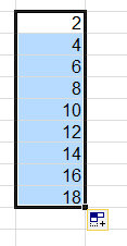
Typing in series of numbers: If your numbers go up by a standard progression, such as 1,2,3,4,… or 2,4,6,8… etc., you can try this trick rather than typing them all in.

• Start typing your numbers in the column
• Highlight your numbers in the column, then look for the small box at the lower right of the last number you’ve typed in the series

• Place your cursor on that box so that the cursor marker turns into a small cross (+)
• Drag that cross down the column and excel will fill in the next numbers in your series

“Locking” or “freezing” a heading in place so you can scroll through your document without losing your headings or row titles:

• Click on the “view” tab
• Click on the “freeze panes” drop-down menu
• Choose which parts of the data set you want to “freeze” and click on that

Copying and pasting formula cells

If you need to take the average or apply a formula to multiple rows or columns of data, you do not need to type it in for every case. If you copy and paste it over a number of cells, Excel automatically advances the cell number for you so that your operation applies to the new cell. For examples, see the hints in the Arithmetic functions sections given in the previous pages.