Many familiar physical quantities can be specified completely by giving a single number and the appropriate unit. For example, “a class period lasts 50 min” or “the gas tank in my car holds 65 L” or “the distance between two posts is 100 m.” A physical quantity that can be specified completely in this manner is called a scalar quantity. Scalar is a synonym of “number.” Time, mass, distance, length, volume, temperature, and energy are examples of scalar quantities.
Scalar quantities that have the same physical units can be added or subtracted according to the usual rules of algebra for numbers. For example, a class ending 10 min earlier than 50 min lasts (50 min – 10 min) = 40 min. Similarly, a 60-cal serving of corn followed by a 200-cal serving of donuts gives (60 cal + 200 cal) = 260 cal of energy. When we multiply a scalar quantity by a number, we obtain the same scalar quantity but with a larger (or smaller) value. For example, if yesterday’s breakfast had 200 cal of energy and today’s breakfast has four times as much energy as it had yesterday, then today’s breakfast has 4(200 cal) = 800 cal of energy. Two scalar quantities can also be multiplied or divided by each other to form a derived scalar quantity. For example, if a train covers a distance of 100 km in 1.0 h, its speed is 100.0 km/1.0 h = 27.8 m/s, where the speed is a derived scalar quantity obtained by dividing distance by time.
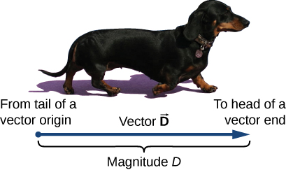
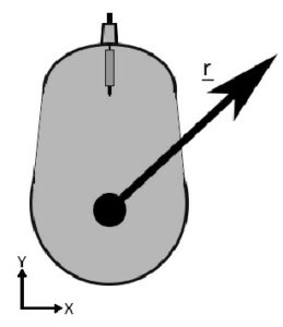
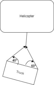
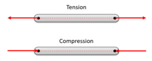
Many physical quantities, however, cannot be described completely by just a single number of physical units. For example, when the U.S. Coast Guard dispatches a ship or a helicopter for a rescue mission, the rescue team must know not only the distance to the distress signal, but also the direction from which the signal is coming so they can get to its origin as quickly as possible. Physical quantities specified completely by giving a number of units (magnitude) and a direction are called vector quantities. Examples of vector quantities include displacement, velocity, position, force, and torque. In the language of mathematics, physical vector quantities are represented by mathematical objects called vectors. We can add or subtract two vectors, and we can multiply a vector by a scalar or by another vector, but we cannot divide by a vector. The operation of division by a vector is not defined.
Source: University Physics Volume 1, OpenStax CNX https://courses.lumenlearning.com/suny-osuniversityphysics/chapter/2-1-scalars-and-vectors
Basically: a scalar has only magnitude, whereas a vector has magnitude and direction.
Application: I might have gone for a 4 km walk (scalar), but whether I walked in a straight line, took turns, or went 2 km out and turned around to walk 2 km back would tell me a lot more information (vector).
Looking ahead: We will talk about this again in sections 1.3 on vectors and in sections 1.4 and 1.5 on dot products and cross products.
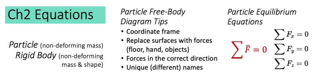
1st Law:
Newton’s first law states that: “A body at rest will remain at rest unless acted on by an unbalanced force. A body in motion continues in motion with the same speed and in the same direction unless acted upon by an unbalanced force.”
This law, also sometimes called the “law of inertia”, means that bodies maintain their current velocity unless a force is applied to change that velocity. If an object is at rest with zero velocity, it will remain at rest until some force begins to change that velocity, and if an object is moving at a set speed and in a set direction, it will remain at that same velocity until some force begins to change that velocity.
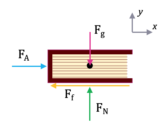
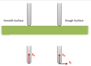
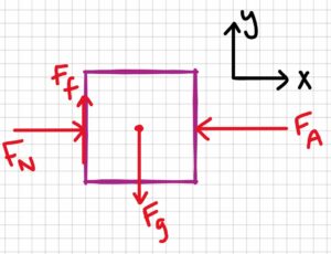
Net Forces: It is important to note that the net force is what will cause a change in velocity. The net force is the sum of all forces acting on the body. For example, we can imagine gently pushing on the rock in the figure below and observing that the rock does not move. This is because we will have a friction force equal in magnitude and opposite in direction opposing our gentle pushing force. The sum of these two forces will be equal to zero; therefore, the net force is zero, and the change in velocity is zero.
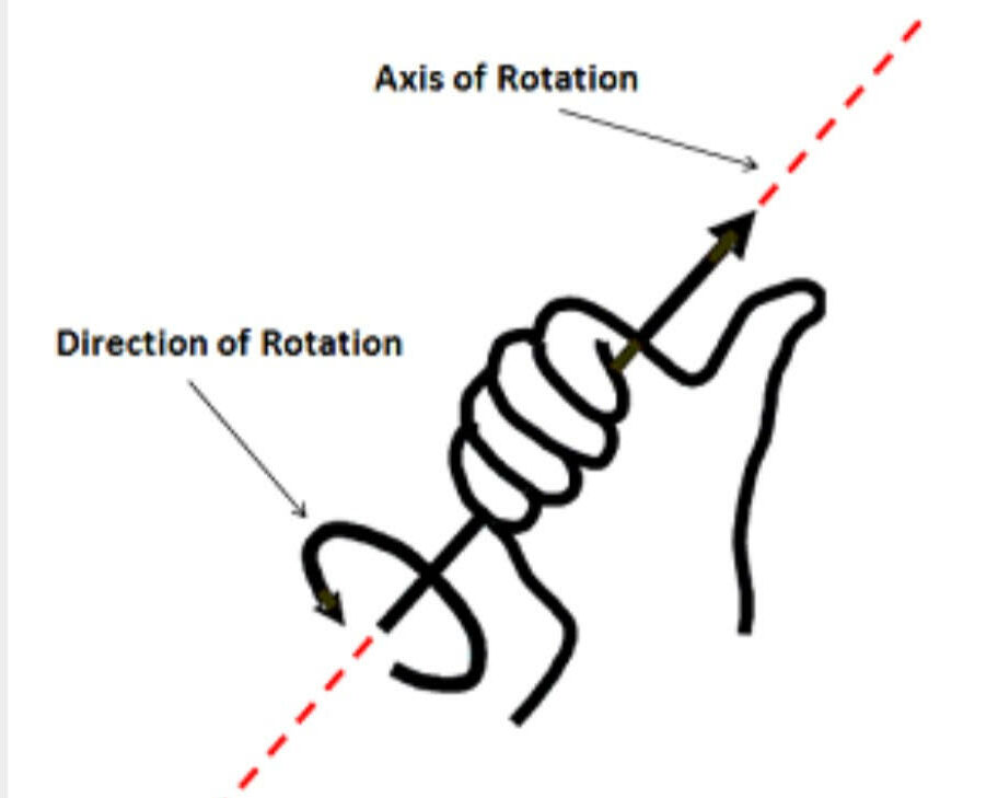
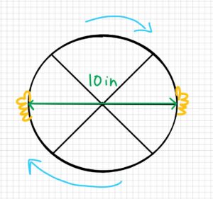
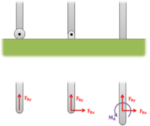
Rotational Motion: Newton’s first law also applies to moments and rotational velocities. A body will maintain its current rotational velocity until a net moment is exerted to change that rotational velocity. This can be seen in things like toy tops, flywheels, stationary bikes, and other objects that will continue spinning once started until brakes or friction stop them.
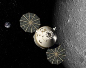
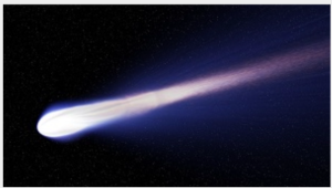
In the absence of friction in space, this space capsule will maintain its current velocity until some outside force causes that velocity to change. Public Domain image by NASA.
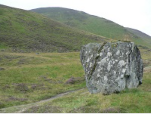
This rock is at rest with zero velocity and will remain at rest until a net force causes the rock to move. The net force on the rock is the sum of any force pushing the rock and the friction force of the ground on the rock opposing that force. Image by Liz Gray CC-BY-SA 2.0.

In the absence of friction, this spinning top would continue to spin forever, but the small frictional moment exerted at the point of contact between the top and the ground will slow the tops spinning over time. Image by Carrotmadman6 CC-BY-2.0
Source: Engineering Mechanics, Jacob Moore et al., Mechanics Map – Newton’s First Law
2nd Law:
Newton’s second law states that: “When a net force acts on any body with mass, it produces an acceleration of that body. The net force will be equal to the mass of the body times the acceleration of the body.”

You will notice that the force and the acceleration in the equation above have an arrow above them. This means that they are vector quantities, having both a magnitude and a direction. Mass, on the other hand, is a scalar quantity having only a magnitude. Based on the above equation, you can infer that the magnitude of the net force acting on the body will be equal to the mass of the body times the magnitude of the acceleration, and that the direction of the net force on the body will be equal to the direction of the acceleration of the body.
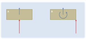
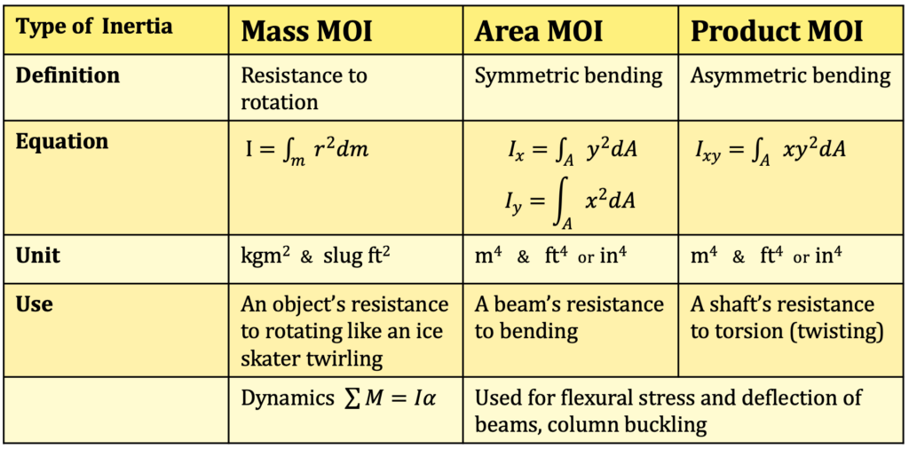
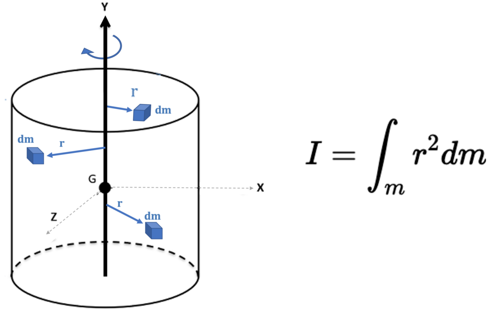
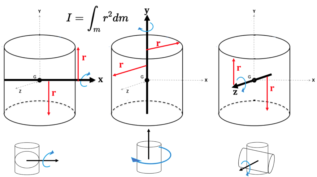
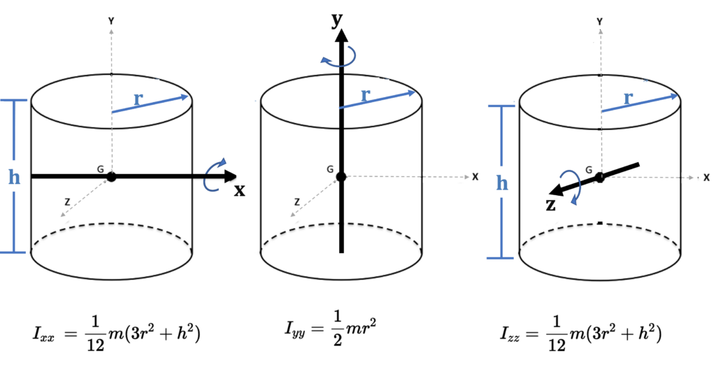
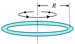
Rotational Motion: Newton’s second law also applies to moments and rotational velocities. The revised version of the second law equation states that the net moment acting on the object will be equal to the mass moment of inertia of the body about the axis of rotation (I) times the angular acceleration of the body.

You should again notice that the moment and the angular acceleration of the body have arrows above them, indicating that they are vector quantities with both a magnitude and direction. The mass moment of inertia, on the other hand, is a scalar quantity having only a magnitude. The magnitude of the net moment will be equal to the mass moment of inertia times the magnitude of the angular acceleration, and the direction of the net moment will be equal to the direction of the angular acceleration.
Source: Engineering Mechanics, Jacob Moore et al., Mechanics Map – Newton’s Second Law
3rd Law:
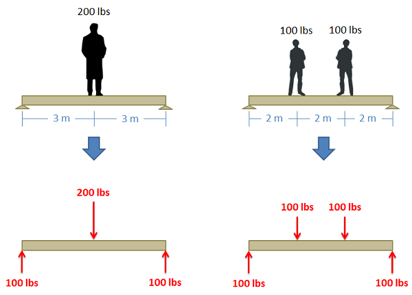
Newton’s Third Law states, “For any action, there is an equal and opposite reaction.” By “action,” Newton meant a force, so for every force one body exerts on another body, that second body exerts a force of equal magnitude but opposite direction back on the first body. Since all forces are exerted by bodies (either directly or indirectly), all forces come in pairs, one acting on each of the bodies interacting.
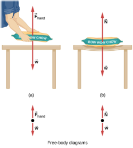
Though there may be two equal and opposite forces acting on a single body, it is important to remember that for each of the forces, a Third Law pair acts on a separate body. This can sometimes be confusing when there are multiple Third Law pairs at work. Below are some examples of situations where multiple Third Law pairs occur.
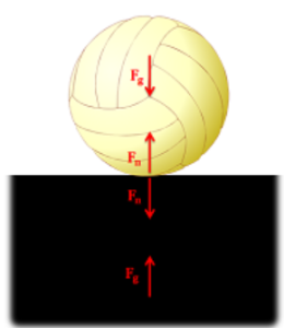
This volleyball resting on a surface has two pairs of Third Law forces. The first consists of the gravitational forces (one force on the ball and one force on the ground). The second consists of the normal forces at the point of contact (one force on the ball and one force on the ground). Image adapted from Public Domain image, no author listed.

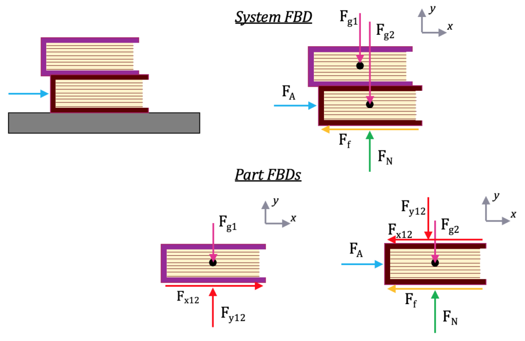
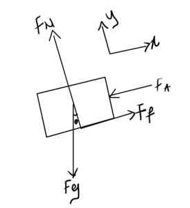
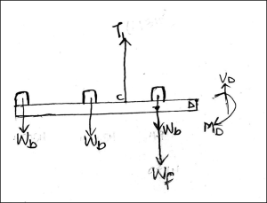
If we ignore the weight of the two objects, this clamp will also have two pairs of Third Law forces. The first will be a set of normal forces at the top point of contact (one force on the wood and one force on the clamp) and the second will be another set of normal forces at the bottom point of contact (one force on the wood and one force on the clamp) Image adapted from Public Domain image, no author listed.
Source: Engineering Mechanics, Jacob Moore et al., Mechanics Map – Newton’s Third Law
Basically: These 3 laws form the foundation of statics and dynamics. It makes our problems interesting! In statics, we don’t do a lot with rotation.
- 1st law: the motion of an object won’t change unless there is a force to cause the change.
- 2nd law: Combination of all forces = mass * acceleration
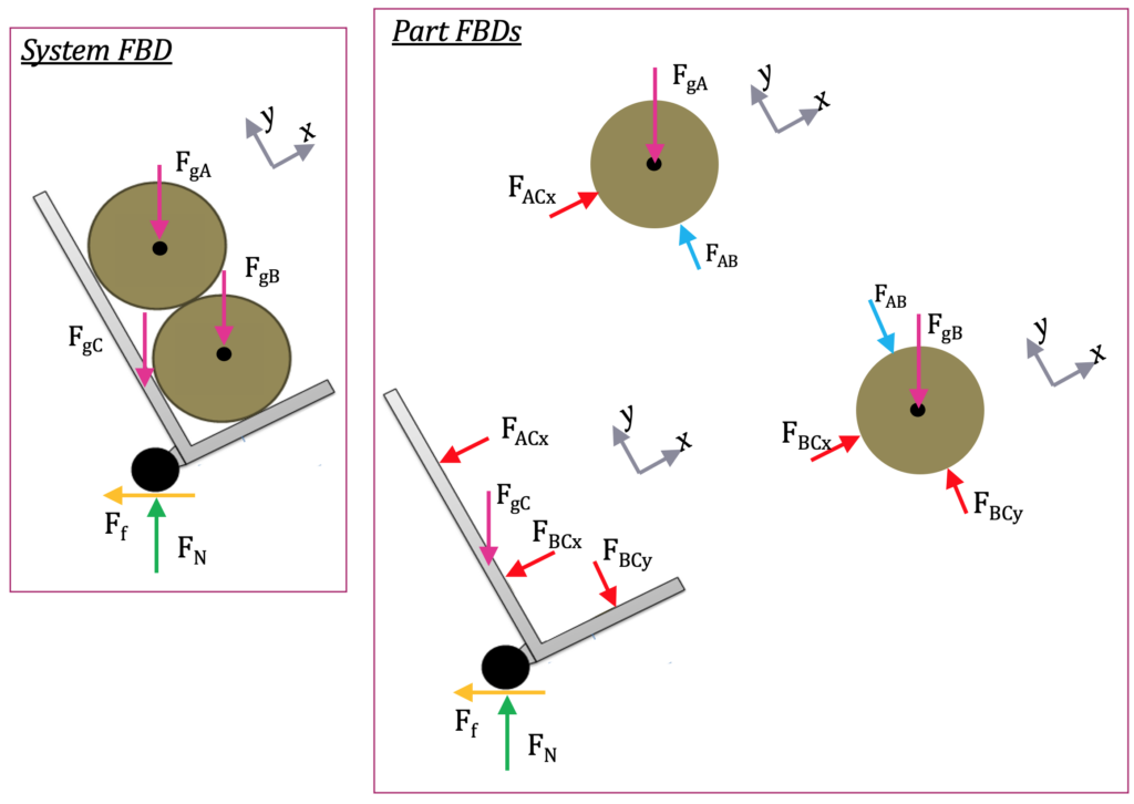
- 3rd law: A system of interacting objects can be split up into parts, where forces are used to model the other part. Forces are equal (same size) and opposite (their directions cancel out – one up, one down
Application: 1st law: a rock rolling down the hill will keep going unless it hits a tree. 2nd law: the amount of forces on the rock and how massive (heavy) it is will determine how much it is accelerating (or decelerating). 3rd law: the rock is pushing on the ground with the same amount of force as the ground is pushing on the rock, but in the opposite direction.
Looking ahead: You’ll see these concepts again in Ch 7 on Inertia (1st law), Section 2.3 and 4.3 on equillibrium equations (2nd law), Section 4.2 on system free-body diagrams (3rd law).
Giving numerical values for physical quantities and equations for physical principles allows us to understand nature much more deeply than qualitative descriptions alone. To comprehend these vast ranges, we must also have accepted units in which to express them. We shall find that even in the potentially mundane discussion of meters, kilograms, and seconds, a profound simplicity of nature appears: all physical quantities can be expressed as combinations of only seven base physical quantities.
We define a physical quantity either by specifying how it is measured or by stating how it is calculated from other measurements. For example, we might define distance and time by specifying methods for measuring them, such as using a meter stick and a stopwatch. Then, we could define average speed by stating that it is calculated as the total distance traveled divided by time of travel.
Measurements of physical quantities are expressed in terms of units, which are standardized values. For example, the length of a race, which is a physical quantity, can be expressed in units of meters (for sprinters) or kilometers (for distance runners). Without standardized units, it would be extremely difficult for scientists to express and compare measured values in a meaningful way.
Two major systems of units are used in the world: SI units (for the French Système International d’Unités), also known as the metric system, and English units (also known as the customary or imperial system). English units were historically used in nations once ruled by the British Empire and are still widely used in the United States. English units may also be referred to as the foot–pound–second (fps) system, as opposed to the centimeter–gram–second (cgs) system.
SI Units: Base and Derived Units
In any system of units, the units for some physical quantities must be defined through a measurement process. These are called the base quantities for that system and their units are the system’s base units. All other physical quantities can then be expressed as algebraic combinations of the base quantities. Each of these physical quantities is then known as a derived quantity and each unit is called a derived unit. The choice of base quantities is somewhat arbitrary, as long as they are independent of each other and all other quantities can be derived from them. Typically, the goal is to choose physical quantities that can be measured accurately to a high precision as the base quantities. The reason for this is simple. Since the derived units can be expressed as algebraic combinations of the base units, they can only be as accurate and precise as the base units from which they are derived.
Based on such considerations, the International Standards Organization recommends using seven base quantities, which form the International System of Quantities (ISQ). These are the base quantities used to define the SI base units. The following table lists these seven ISQ base quantities and the corresponding SI base units.
| ISQ Base Quantity | SI Base Unit |
| Length | Meter (m) |
| Mass | Kilogram (kg) |
| Time | Second (s) |
| Electrical current | Ampere (A) |
| Thermodynamic temp. | Kelvin (K) |
| Amount of substance | Mole (mol) |
| Luminous intensity | Candela (cd) |
You are probably already familiar with some derived quantities that can be formed from the base quantities. For example, the geometric concept of area is always calculated as the product of two lengths. Thus, area is a derived quantity that can be expressed in terms of SI base units using square meters (m x m = m2).
Similarly, volume is a derived quantity that can be expressed in cubic meters (m3). Speed is length per time; so in terms of SI base units, we could measure it in meters per second (m/s). Volume mass density (or just density) is mass per volume, which is expressed in terms of SI base units such as kilograms per cubic meter (kg/m3). Angles can also be thought of as derived quantities because they can be defined as the ratio of the arc length subtended by two radii of a circle to the radius of the circle. This is how the radian is defined. Depending on your background and interests, you may be able to come up with other derived quantities, such as the mass flow rate (kg/s) or volume flow rate (m3/s) of a fluid, electric charge (A·s), mass flux density kg/(m2·s), and so on. We will see many more examples throughout this text. For now, the point is that every physical quantity can be derived from the seven base quantities, and the units of every physical quantity can be derived from the seven SI base units.
Source: University Physics Volume 1, OpenStax CNX, https://courses.lumenlearning.com/suny-osuniversityphysics/chapter/1-2-units-and-standards/
While most Canadian companies use SI, much manufacturing still uses English units, so it’s important for you to be familiar with them. What is a big number in feet? What is small? It’s important to know. The most important advice is to stay in one unit system. So, if you are doing a homework problem that has a mixture, convert to one system to be consistent. Challenge yourself to try the one you aren’t comfortable with. Here is a table of the most common quantities that we’ll use in this class:
| Quantity | SI Unit | English |
| Length | m (meter), km (kilometer), mm (milimeter) | ft (foot), mi (mile), in (inch) |
| Mass | kg (kilogram) | slug |
| Force | N (Newton) | lb (pound) |
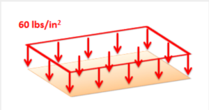
| Pressure | Pa (Pascal) = N/m2 | psi (pound per square inch) = lb/in2 |
Very helpful additional information about units is at this webpage:
https://www.physics.nist.gov/cuu/Units/index.html
Basically: Units give us a standard so we can use the same language to describe a concept.
Application: In 1999, after taking 286 days for NASA Mars Orbiter satellite to get to Mars, a conversion error between N and lb caused the $125 million satellite to be lost, forever. Click here for more fun conversion error stories. If you want to design ANYTHING, you need to be sure everyone involved is using the same unit system.
Looking Ahead: The next section (1.1.4) will look at converting the units back and forth between the two systems.
It is often necessary to convert from one unit to another. For example, if you are reading a European cookbook, some quantities may be expressed in units of liters and you need to convert them to cups. Or perhaps you are reading walking directions from one location to another and you are interested in how many miles you will be walking. In this case, you may need to convert units of feet or meters to miles.
Let’s consider a simple example of how to convert units. Suppose we want to convert 80 m to kilometers. The first thing to do is to list the units you have and the units to which you want to convert. In this case, we have units in meters and we want to convert to kilometers. Next, we need to determine a conversion factor relating meters to kilometers. A conversion factor is a ratio that expresses how many of one unit are equal to another unit. For example, there are 12 in. in 1 ft, 1609 m in 1 mi, 100 cm in 1 m, 60 s in 1 min, and so on. In this case, we know that there are 1000 m in 1 km. Now we can set up our unit conversion. We write the units we have and then multiply them by the conversion factor so the units cancel out, as shown:

Note that the unwanted meter unit cancels, leaving only the desired kilometer unit. You can use this method to convert between any type of unit. Now, the conversion of 80 m to kilometers is simply the use of a metric prefix, as we saw in the preceding section, so we can get the same answer just as easily by noting that
Since “kilo-” means 103, however, using conversion factors is handy when converting between units that are not metric or when converting between derived units, as the following examples illustrate.
Source: University Physics Volume 1, OpenStax CNX, https://courses.lumenlearning.com/suny-osuniversityphysics/chapter/1-3-unit-conversion/
Going back and forth between SI and English will become a very useful skill. If you can memorize km to mi, ft to m, and inches to ft, you’ll be able to communicate better with coworkers. Here are common conversions you’ll need for this course:
| Quantity | SI
| English | Convert |
| Length | 1 km = 1000 m 1 m = 1000 mm | 1 mi = 5,280 ft 1 ft = 12 in | 1 m = 3.28 ft 2.2 km = 1 mi |
| Mass | kg | slug | 1 slug = 14.6 kg |
| Force | N | lb | 1 lb = 4.448 N |
| Pressure | Pa | psi | |
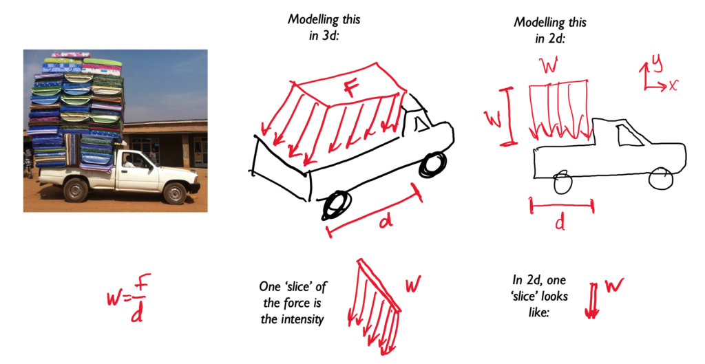
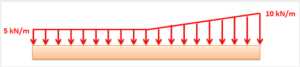
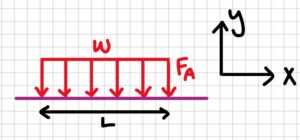
All of the other units that we will encounter will be a mix of these units (intensity w = N/m or lb/ft). One additional conversion that is common is 1 lb = 2.2 kg, though this only works on Earth because it is mixing kg and lb (see next section). For a full table, MechanicsMap has a pdf available: http://mechanicsmap.psu.edu/websites/UnitConversion.pdf
Units outside the SI that are accepted for use with the SI
| | Name | Symbol | Value in SI units | | minute (time) | min | 1 min = 60 s | | hour | h | 1 h = 60 min = 3600 s | | day | d | 1 d = 24 h = 86 400 s | | degree (angle) | ° | 1° = (  /180) rad /180) rad | | minute (angle) |  | 1 = (1/60)° = (/10 800) rad | | second (angle) | | 1 = (1/60) = (/648 000) rad | | liter | L | 1 L = 1 dm3 = 10-3 m3 | | metric ton (a) | t | 1 t = 103 kg | | neper | Np | 1 Np = 1 | | bel (b) | B | 1 B = (1/2) ln 10 Np (c) | | electronvolt (d) | eV | 1 eV = 1.602 18 x 10-19 J, approximately | | unified atomic mass unit (e) | u | 1 u = 1.660 54 x 10-27 kg, approximately | | astronomical unit (f) | au | 1 au = 149 597 870 700 m, exactly | (a) In many countries, this unit is called “tonne.”
(b) The bel is most commonly used with the SI prefix deci: 1 dB = 0.1 B.
(c) Although the neper is coherent with SI units and is accepted by the CIPM, it has not been adopted by the General Conference on Weights and Measures (CGPM, Conférence Générale des Poids et Mesures) and is thus not an SI unit.
(d) The electronvolt is the kinetic energy acquired by an electron passing through a potential difference of 1 V in vacuum. The value must be obtained by experiment, and is therefore not known exactly.
(e) The unified atomic mass unit is equal to 1/12 of the mass of an unbound atom of the nuclide 12C, at rest and in its ground state. The value must be obtained by experiment, and is therefore not known exactly.
(f) The astronomical unit of length was redefined by the XXVIII General Assembly of the International Astronomical Union (Resolution B2, 2012). |
Source: https://www.physics.nist.gov/cuu/Units/outside.html |
| | |
| | |
| | |
| | |
| | |
| | |
| | |
| | |
| | |
| | |
| | |
| | |
| | |
| | |
|
Basically: Different industries use different standards. English is common in the US. SI is standard many other places, however not generally in aerospace.
Application: In 1999, after taking 286 days for NASA Mars Orbiter satellite to get to Mars, a conversion error between N and lb caused the $125 million satellite to be lost, forever. Click here for more fun conversion error stories. If you want to design ANYTHING, you need to be sure everyone involved is using the same unit system.
Looking Ahead: Always always always check what unit you’re using. So many students lose points on homework and the test because they aren’t paying attention to units.
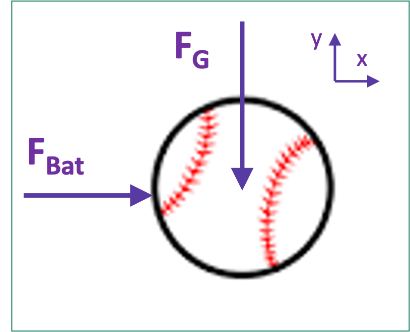
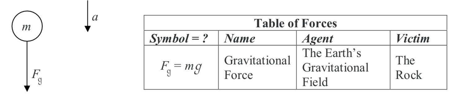
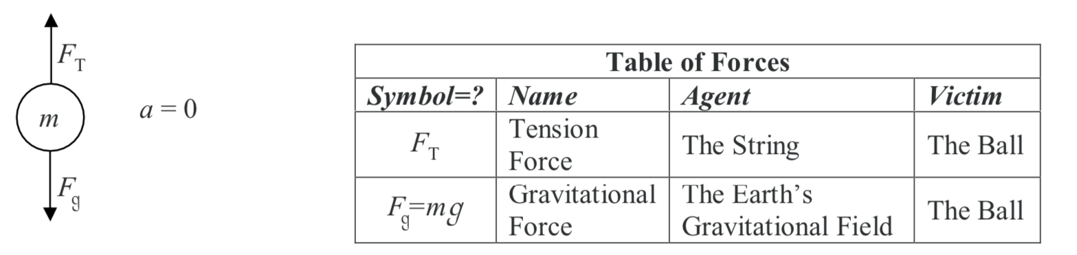
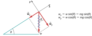
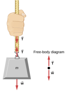
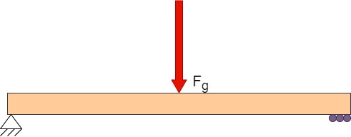
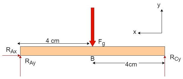
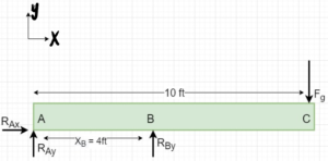
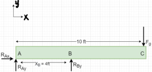
Weight is the force exerted by gravity. While all objects with mass exert an attractive force of gravity on all other objects with mass, that force is usually negligible unless the mass of one of the objects is very large. For an object near the surface of the Earth, we can, to a very good degree of approximation, assume that the only force of gravity on the object is from the Earth. We usually label the force of gravity on an object as Fg. All objects near the surface of the Earth will experience a weight, as long as they have a mass. If an object has a mass, m, and is located near the surface of the Earth, it will experience a force (its weight) that is given by:
where g is the Earth’s “gravitational field” vector and points towards the centre of the Earth. Near the surface of the Earth, the magnitude of the gravitational field is approximately g = 9.81 m/s2. The gravitational field is a measure of the strength of the force of gravity from the Earth (it is the gravitational force per unit mass). The magnitude of the gravitational field is weaker as you move further from the centre of the Earth (e.g. at the top of a mountain, or in Earth’s orbit). The gravitational field is also different on different planets; for example, at the surface of the moon, it is approximately gm = 1.62 m/s2 (six times less) – thus the weight of an object is six times less at the surface of the moon (but its mass is still the same). As we will see, the magnitude of the gravitational field from any spherical body of mass M (e.g a planet) is given by:
where G = 6.67 × 10⁻¹¹ is Newton’s constant of gravity, and r is the distance from the centre of the object.
Although we have not yet introduced the concept of mass, it is worth emphasizing that mass and weight are different (they have different dimensions). Mass is an intrinsic property of an object, whereas weight is a force of gravity that is exerted on that object because it has mass and is located next to another object with mass (e.g. the Earth). On Earth, when we measure our weight, we usually do so by standing on a spring scale, which is designed to measure a force by compressing a spring. We are thus measuring mg, which can easily be related to our mass since, on Earth, weight and mass are related by a factor of g = 9.81 m/s2; this is usually what leads to the confusion between mass and weight.
Source: Introductory Physics, Ryan Martin et al., https://openlibrary.ecampusontario.ca/catalogue/item/?id=4c3c2c75-0029-4c9e-967f-41f178bebbbb page 106
In the English language, the words ‘mass’ and ‘weight’ are used interchangeably. A person might say, “I weigh 50 kg”, but in statics language, that’s wrong! Or more accurately, that language isn’t precise enough for statics.
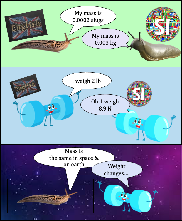
An object’s mass is the same whether they are on the moon, Mars, or Earth. However, their weight changes because the constant of gravity with which that planet is pulling changes (see above description comparing the moon and Earth).
g = 9.81 m/s2 (SI) and g = 32.2 ft/s2 (English)

Weight = mass * gravitational constant
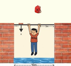
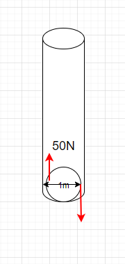
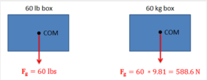
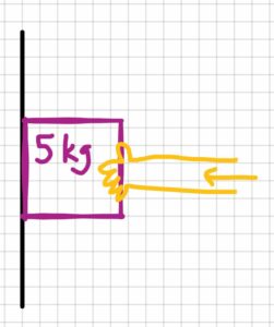
Units of mass are kg (SI) or slugs (English), whereas units of weight/force are N (SI) or lb (English). Because ‘slugs’ is such an odd, unfamiliar unit, the graphic on the left uses real slugs to help you remember to say “my mass is 50 kg (or 3.43 slugs)” or “I weigh 490 N (or 110 lb)”.
While most Canadian companies use SI units, it’s important to be familiar with English, so you should learn slugs. You don’t want to be excluded from a conversation at your future job.
Note lbm (pound-mass) is not used in this book, though some textbooks use it as a mass value. When lb is used, it is assumed to be lbf (pound-force).
Basically: Mass and force are two different quantities. Mass is in kg (SI) or slug (English), and weight is in N (SI) and lb (English).
Application: Mass stays the same, but weight changes from the Earth to the moon.
Looking ahead: This will become very important when we look at forces in Section 4.1.
Right triangle: a triangle containing a 90° angle.
Pythagorean theorem: a relation among the three sides of a right triangle which states that the square of the hypotenuse is equal to the sum of the squares of the other two sides (legs).
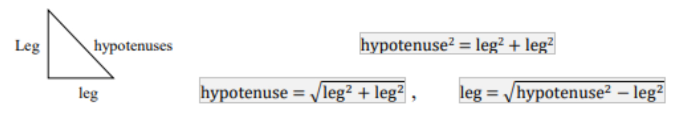
Using the Pythagorean theorem can find the length of the missing side in a right triangle.
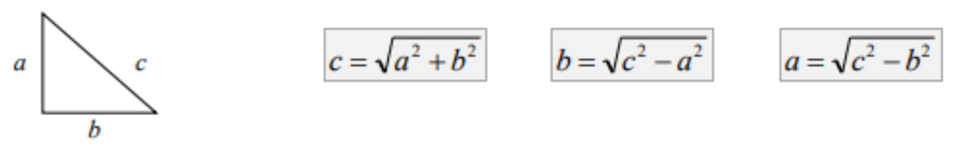
▪ c is the longest side of the triangle (hypotenuse).
▪ Other two sides (legs) of the triangle a and b can be exchanged.
Source: Key Concepts of Intermediate Level Math, Meizhong Wang and the College of New Caledonia, https://openlibrary.ecampusontario.ca/catalogue/item/?id=d8bdc88b-5439-4652-b4bb-2948f0d5c625, page 136.
A special case of the right triangle is called a 3-4-5 triangle, or a Pythagorean triple. The two short sides are 3 and 4, and the hypotenuse is 5! Many of your homework problems will use this coincidence, so you can save on the math by remembering 3-4-5 triangles: 32 + 42 = 52, 9 + 16 = 25. Wow!
Basically: The Pythagorean theorem will help you find a lot of information throughout this course. The longest side c2 = a2 + b2
Application: If I have a 6 ft ladder leaned up against a wall whose base is 2 ft from the wall, the Pythagorean theorem helps you to calculate the vertical height of the ladder (b2 = 62 – 22 ).
Looking Ahead: You’ll use this to help find geometrical aspects of the problems, especially when we get into trusses in Ch 5.
The Six Basic Trigonometric Functions
Trigonometric functions allow us to use angle measures, in radians or degrees, to find the coordinates of a point on any circle—not only on a unit circle—or to find an angle given a point on a circle. They also define the relationship among the sides and angles of a triangle.
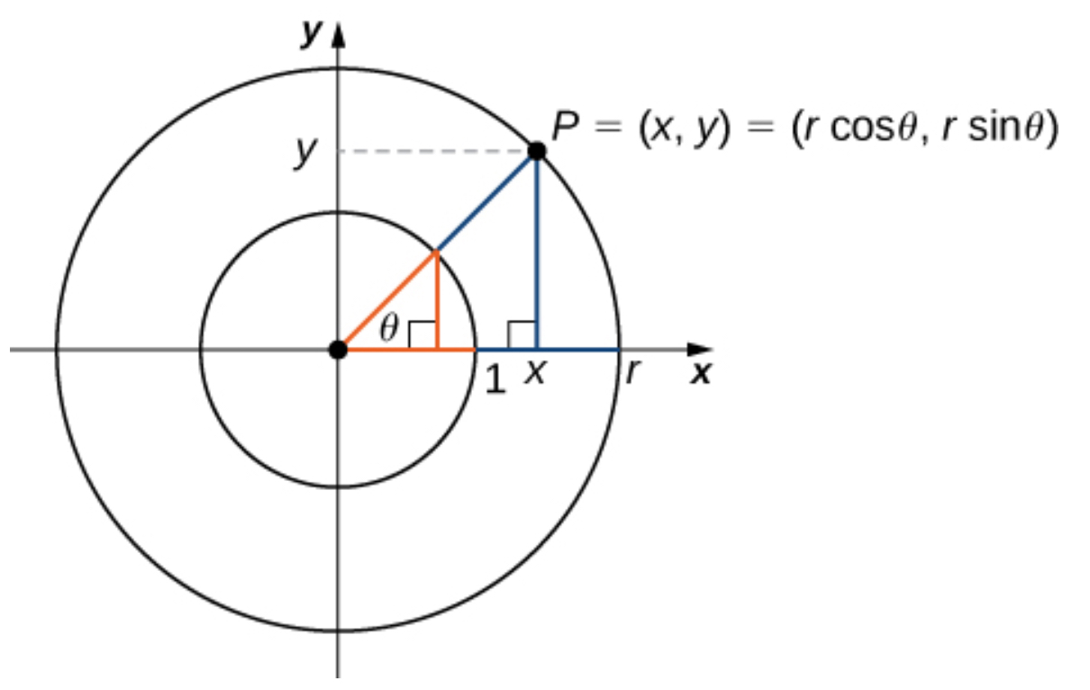
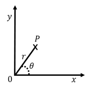
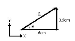
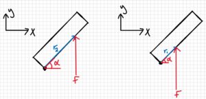
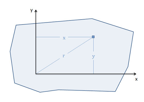
To define the trigonometric functions, first consider the unit circle centred at the origin and a point P = (x,y) on the unit circle. Let θ be an angle with an initial side that lies along the positive x-axis and with a terminal side that is the line segment OP. We can then define the values of the six trigonometric functions for θ in terms of the coordinates x and y.
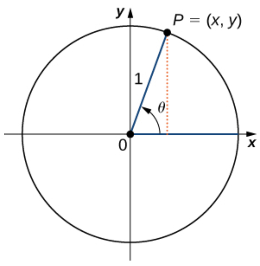
Let P=(x,y) be a point on the unit circle centered at the origin O. Let θ be an angle with an initial side along the positive x-axis and a terminal side given by the line segment OP. The trigonometric functions are then defined as
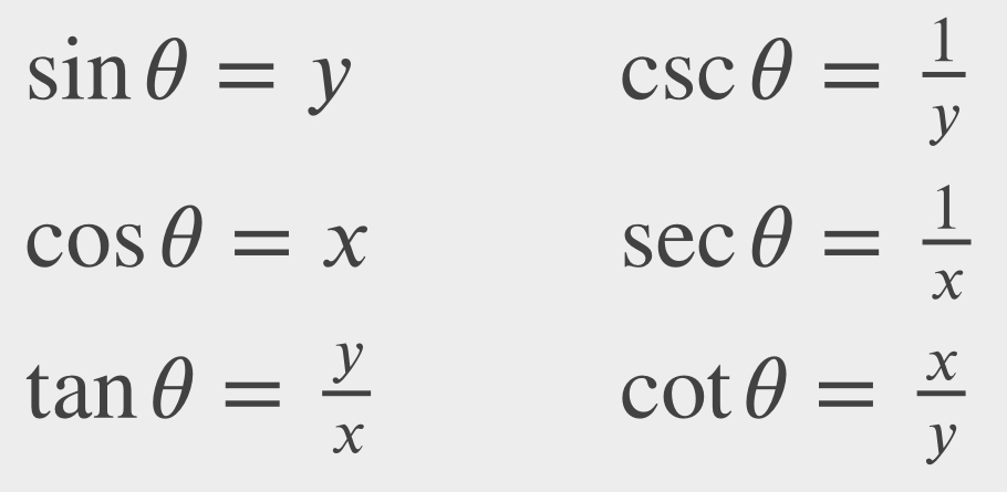
If x=0, secθ and tanθ are undefined. If y=0, then cotθ and cscθ are undefined.
We can see that for a point P=(x,y) on a circle of radius r with a corresponding angle θ,the coordinates x and y satisfy:
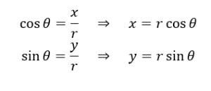
The values of the other trigonometric functions can be expressed in terms of x, y, and r:
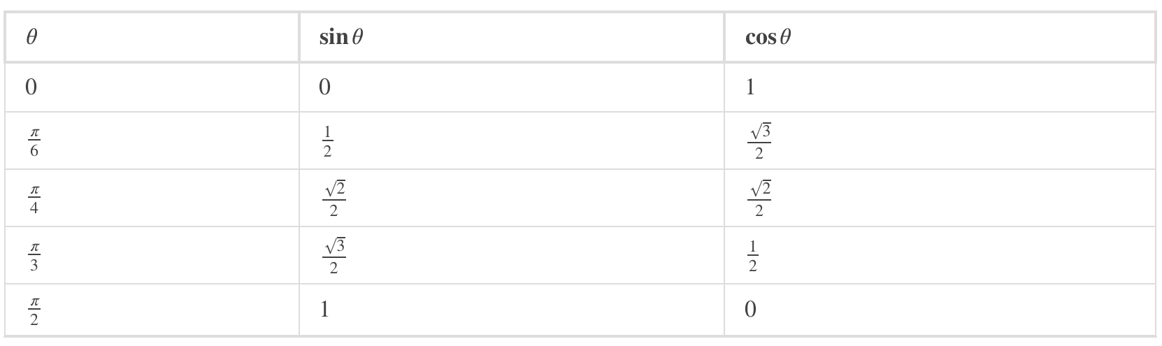
The table below shows the values of sine and cosine at the major angles in the first quadrant. From this table, we can determine the values of sine and cosine at the corresponding angles in the other quadrants. The values of the other trigonometric functions are calculated easily from the values of sinθ and cosθ:
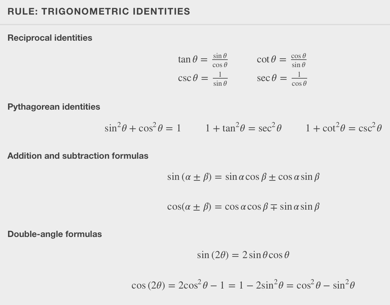
Trigonometric Identities
A trigonometric identity is an equation involving trigonometric functions that is true for all angles θ for which the functions are defined. We can use the identities to help us solve or simplify equations. The main trigonometric identities are listed next.
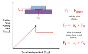
We often refer to this as SOH-CAH-TOA:
- Sine = Opposite / Hypotenuse >> S = O/H >> SOH
- Cosine = Adjacent / Hypotenuse >> C = A / H >> CAH
- Tangent = Opposite / Adjacent >> T = O / A >> TOA
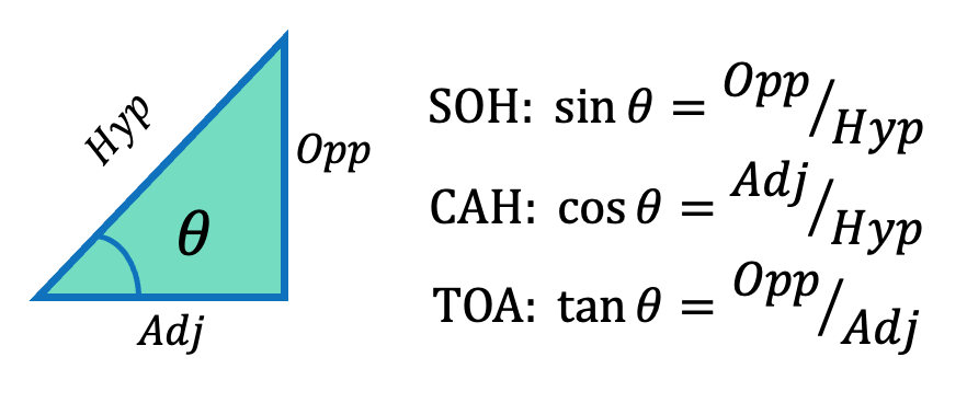
I remember that cos is close – the side that’s close to the angle is cosine. (It kind of rhymes and ‘close’ is a more familiar word than ‘adjacent’).
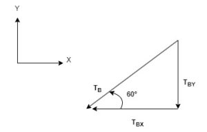
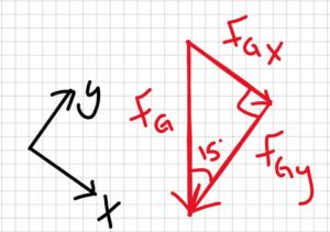
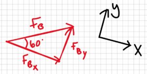
Basically: Trigonometric functions will help you to solve problems. You’ll use SOH-CAH-TOA in many statics problems, whether to componentize a vector or resolve a force.
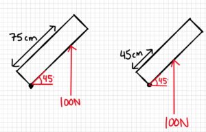
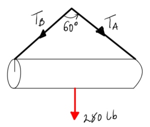
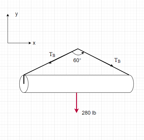
Application: A 6ft ladder leaning up against a house is at a 60-degree angle. We can find the vertical height where the ladder reaches the house by using height = 6 ft * sin 60 degrees. (sin = opp / hyp)
Looking Ahead: Chapter 4 (forces) and Chapter 5 (trusses) will use the calculation of angles a lot.

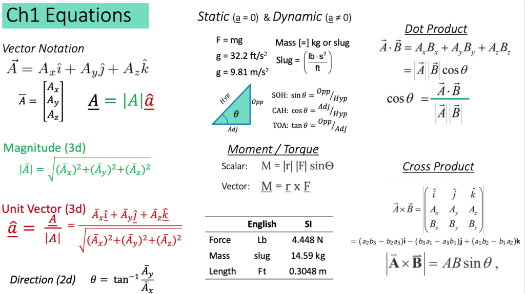
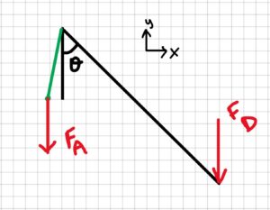
 The dot product is the component of vector A along B ( |A| cos Θ ) times the magnitude (size of B). OR, it’s the component of B on A times the magnitude of A.
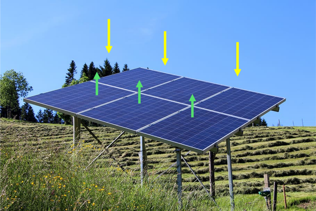
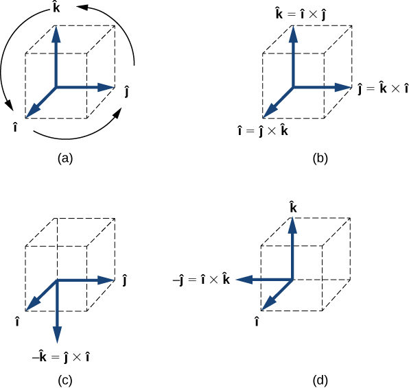
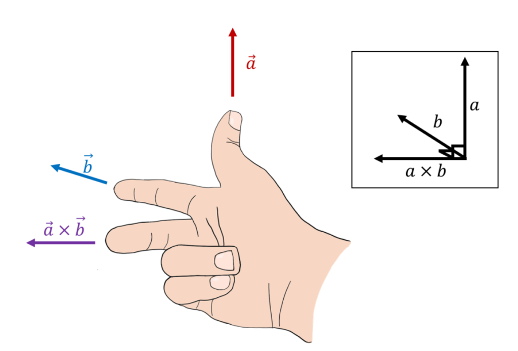
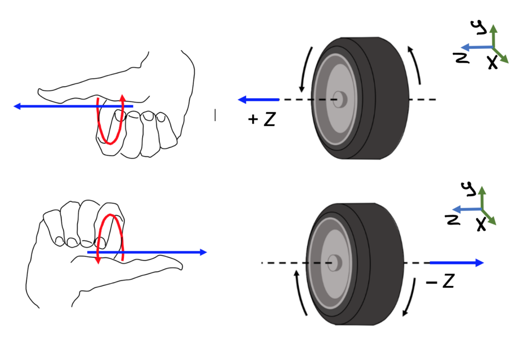
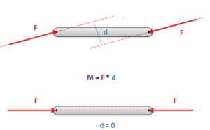
 The black arrow is perpendicular to the grey plane made from blue and red vectors). This is how you will find the amount of torque created from a force, which we will do many times. Also, unlike the dot product,


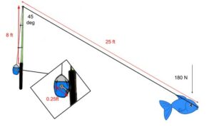
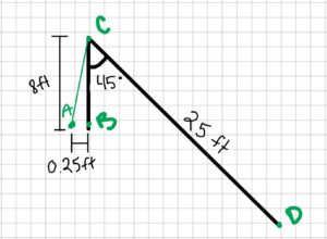


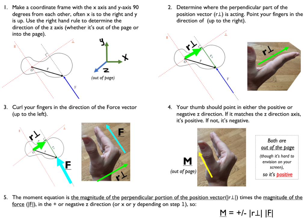

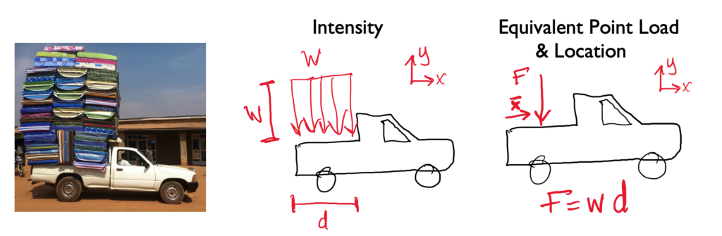
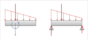
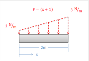
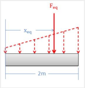
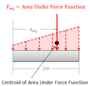
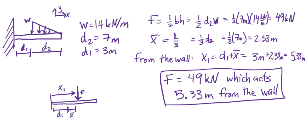
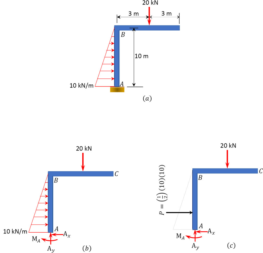
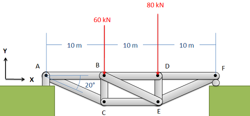
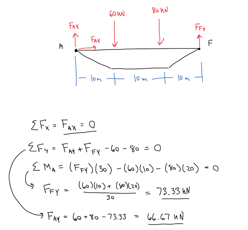
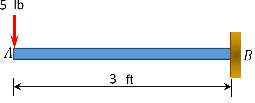
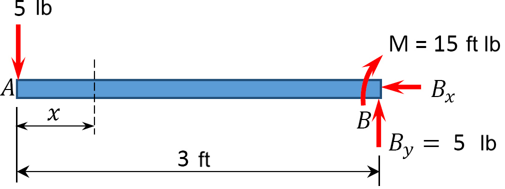
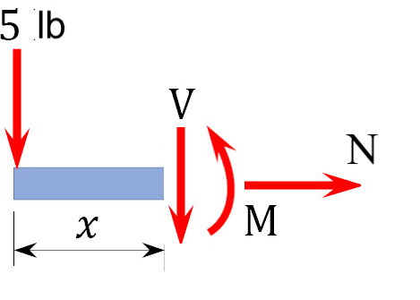
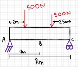
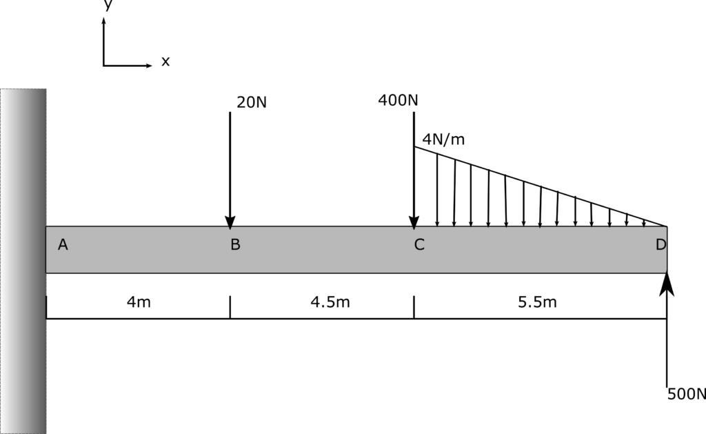
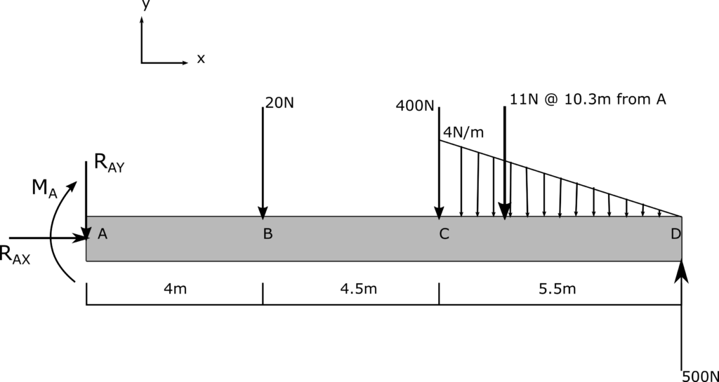
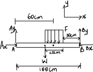
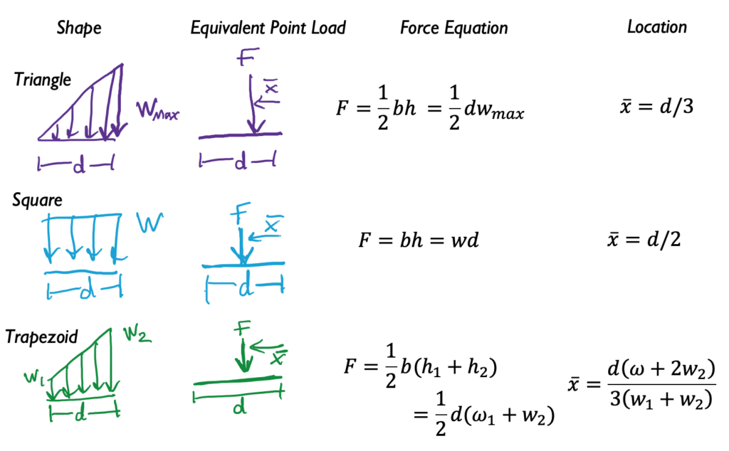 Example 1: Equivalent force and location:
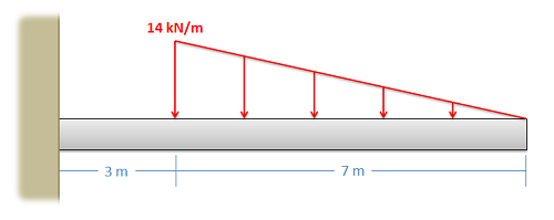


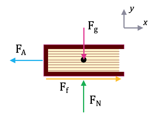


 Source:https://www.omnicalculator.com/physics/normal-force


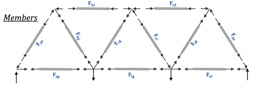
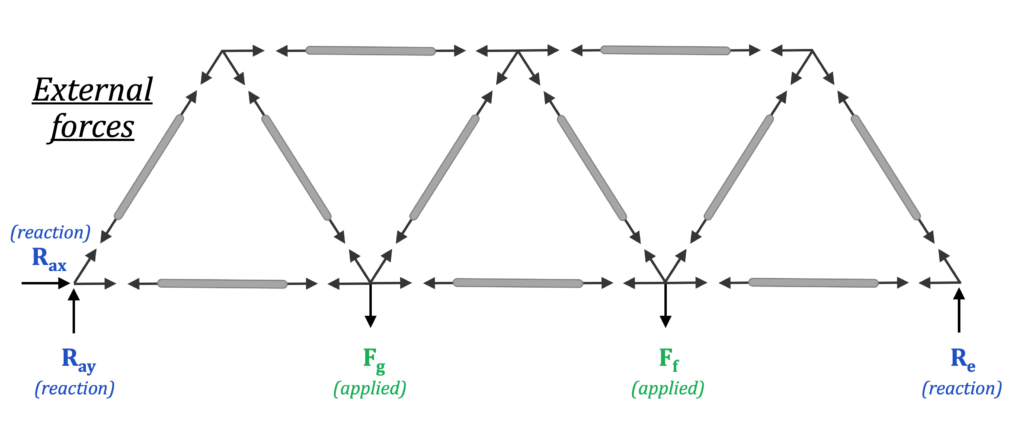
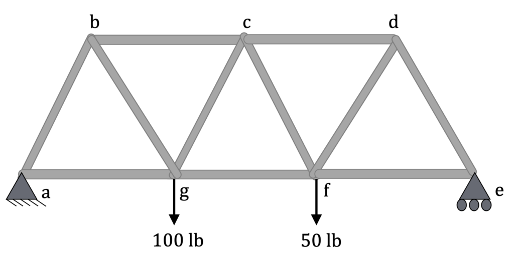
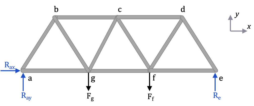
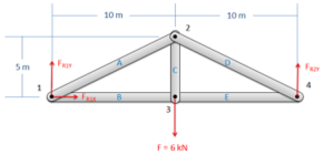
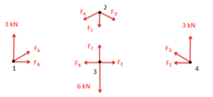
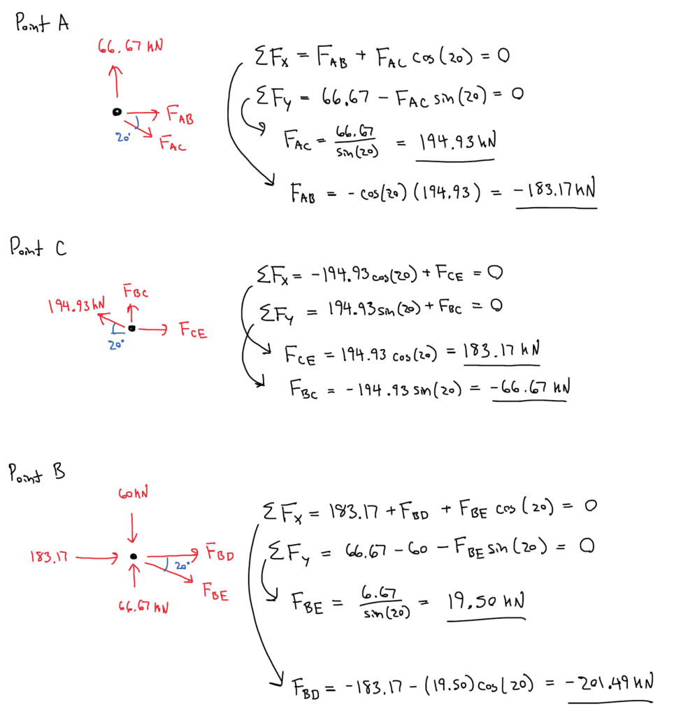
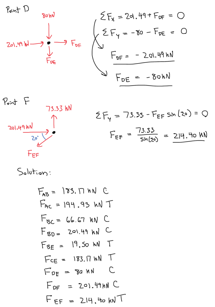
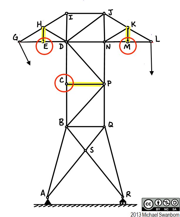
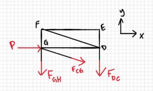
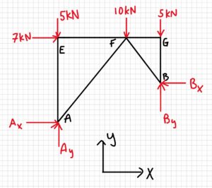
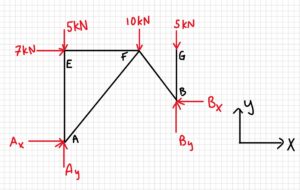
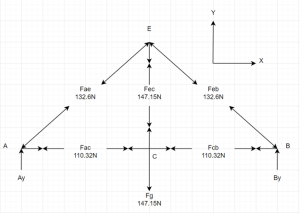
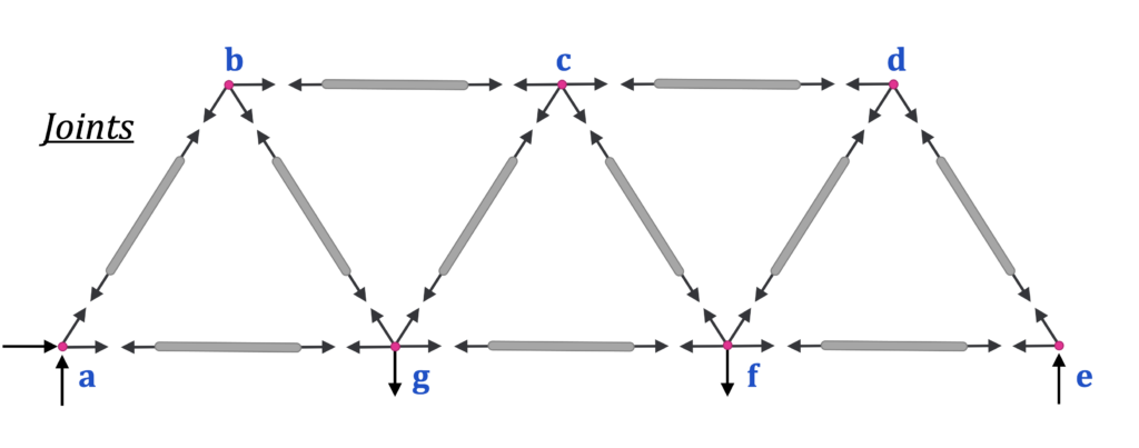 Here is an example of just the joints without the members:


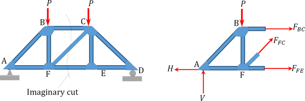
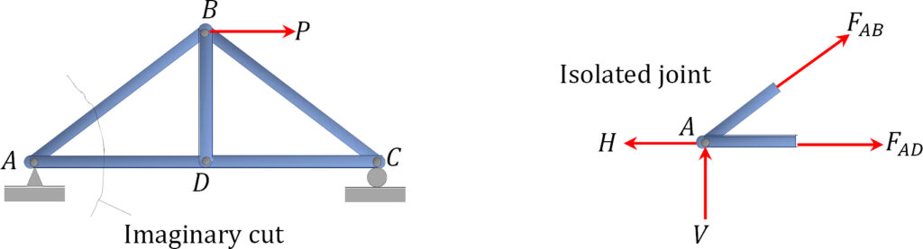
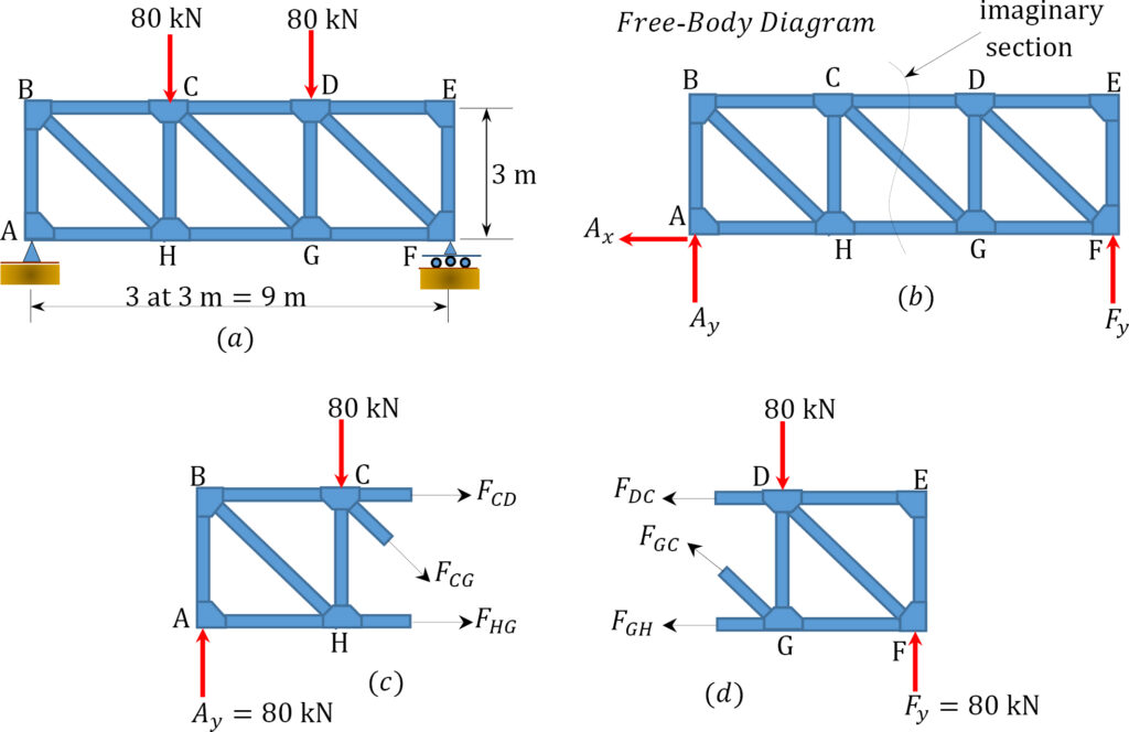


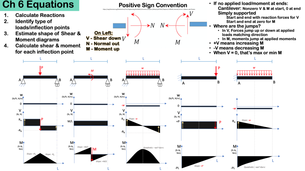
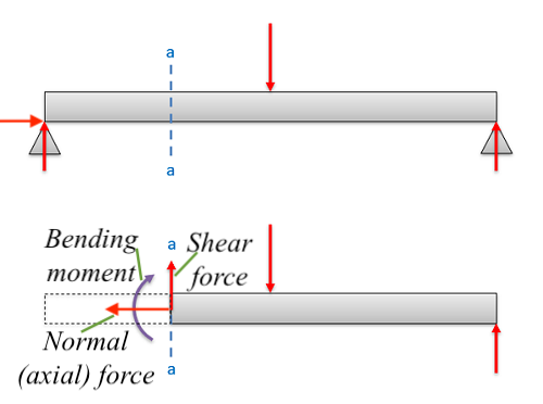

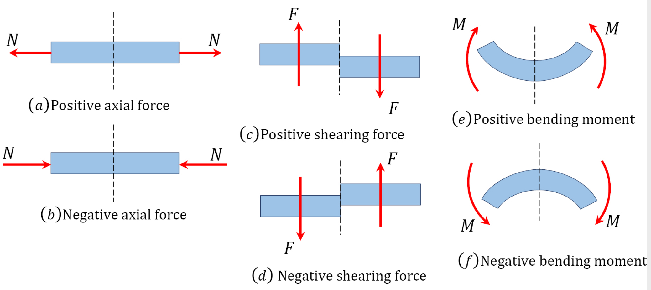
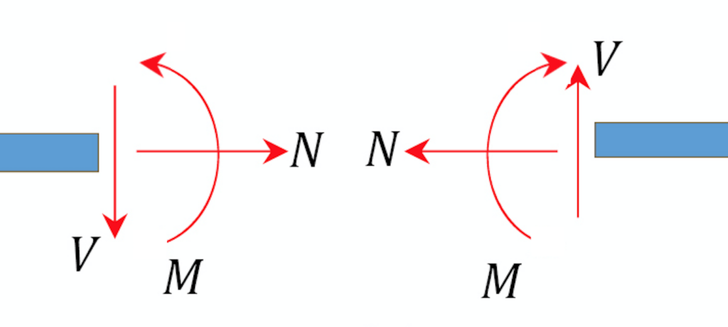
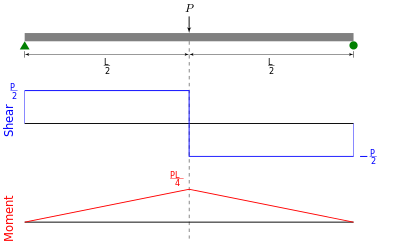
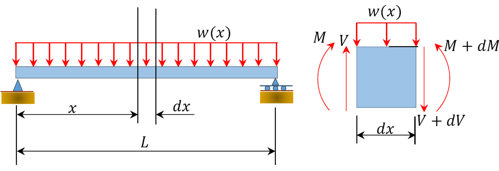

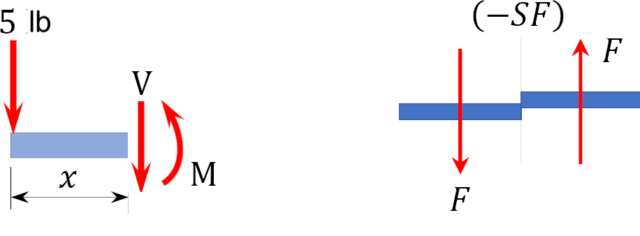
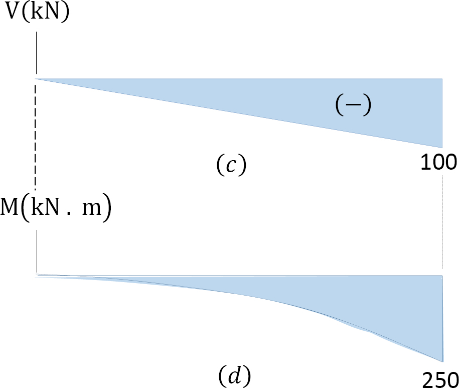
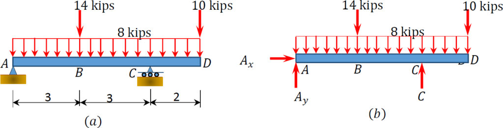
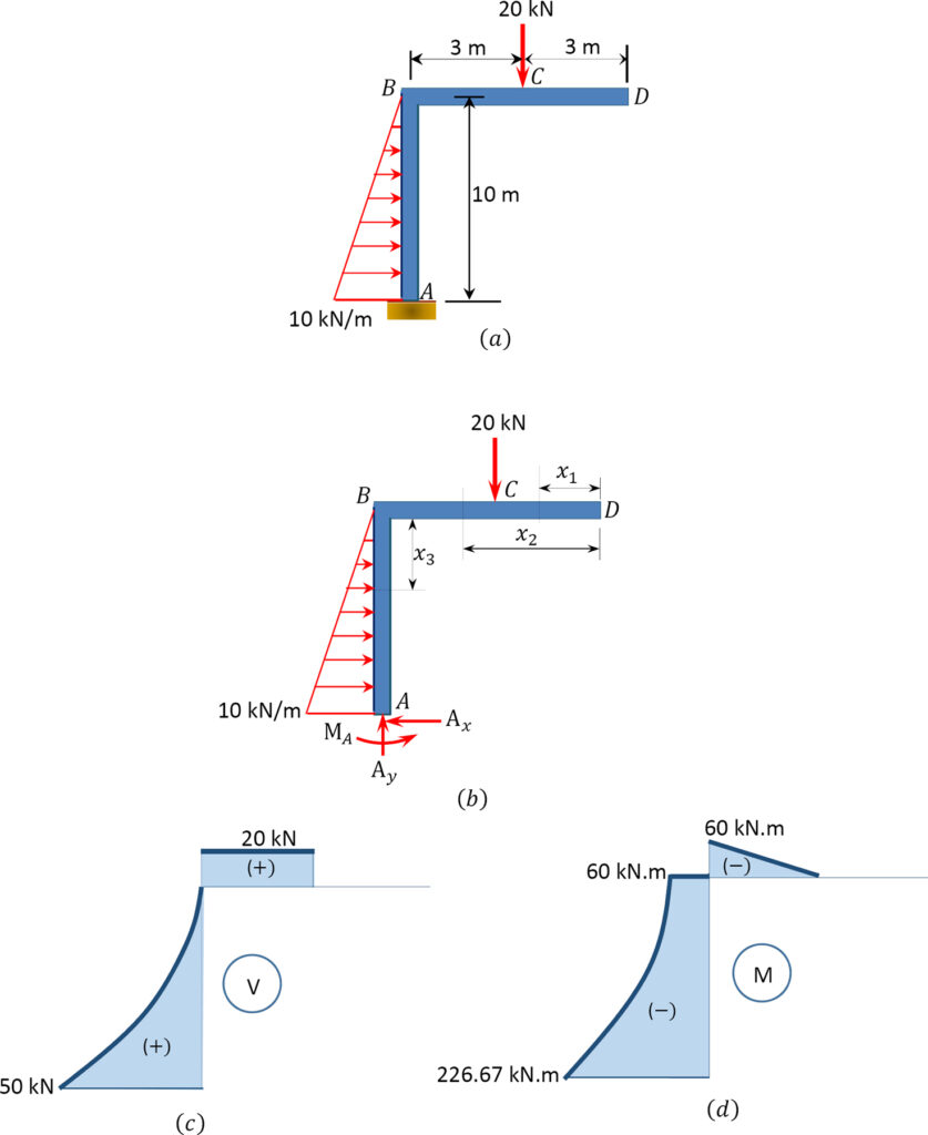
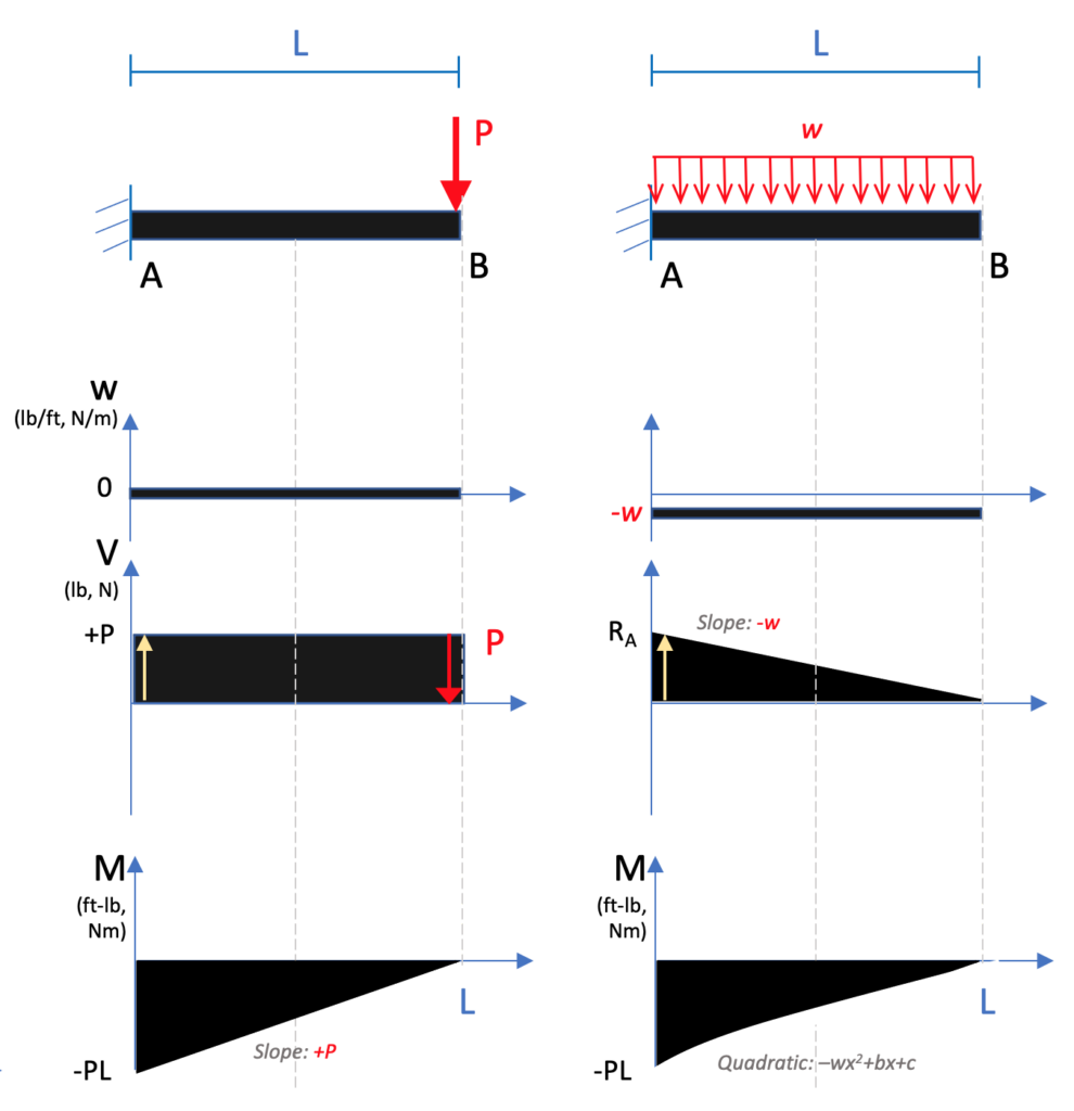
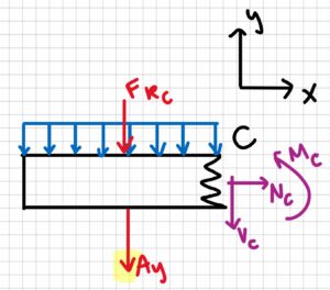
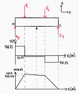
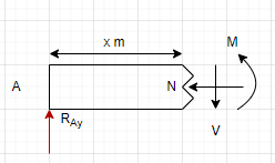
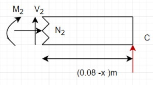
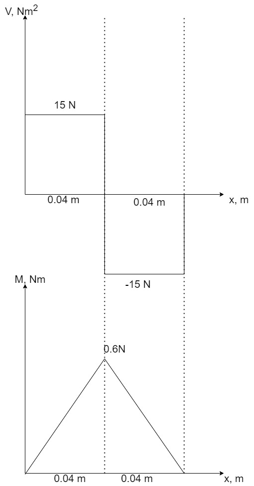
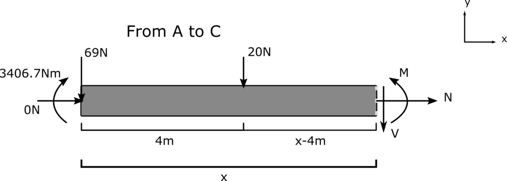
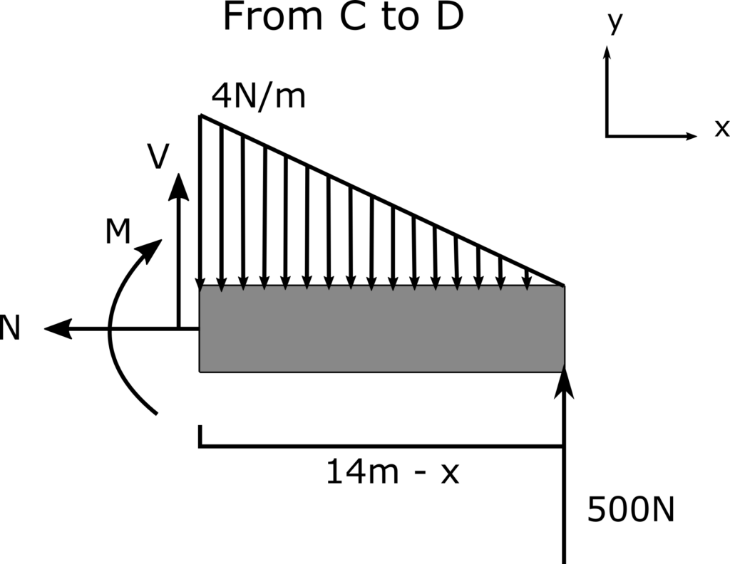
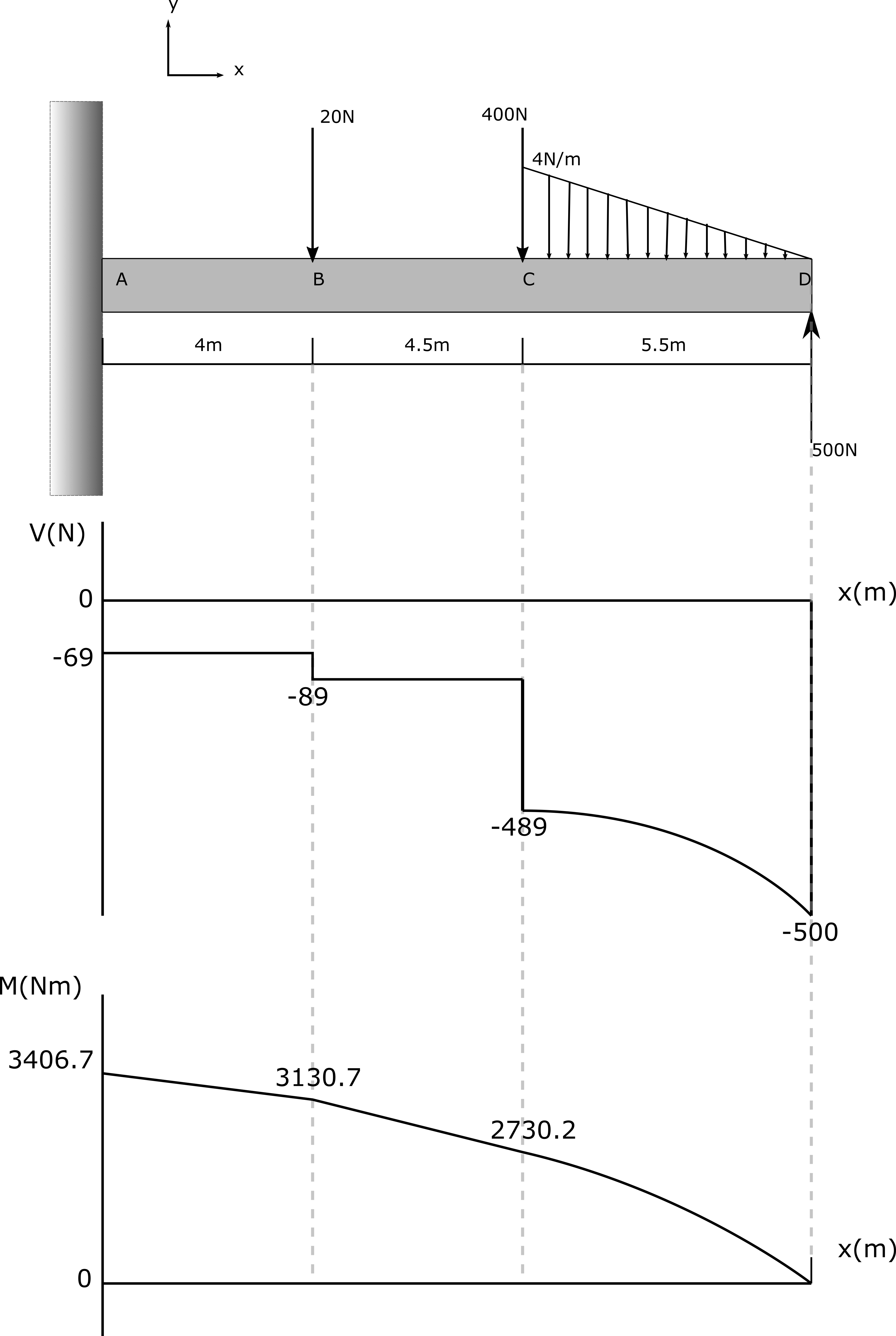
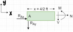
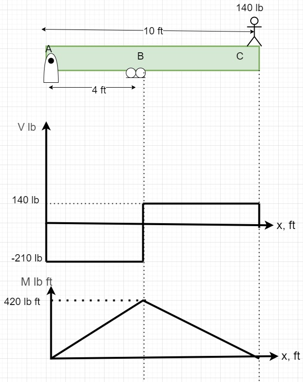
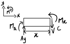
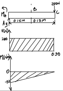
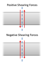 To read the plot, you simply need to find the location of interest from the free body diagram above, and read the corresponding value on the y-axis from your plot. Positive numbers represent an upward internal shearing force to the right of the cross section and a downward force on the left, and negative numbers indicate a downward internal shearing force to the right of the cross section and an upward force on the left. A visual of these forces can be seen in the diagram to the right.
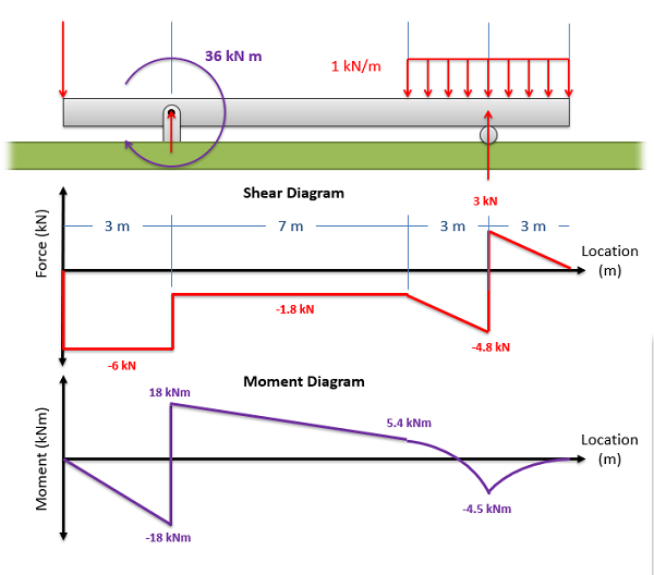
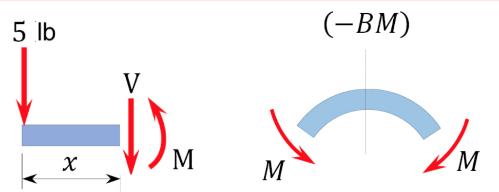
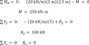
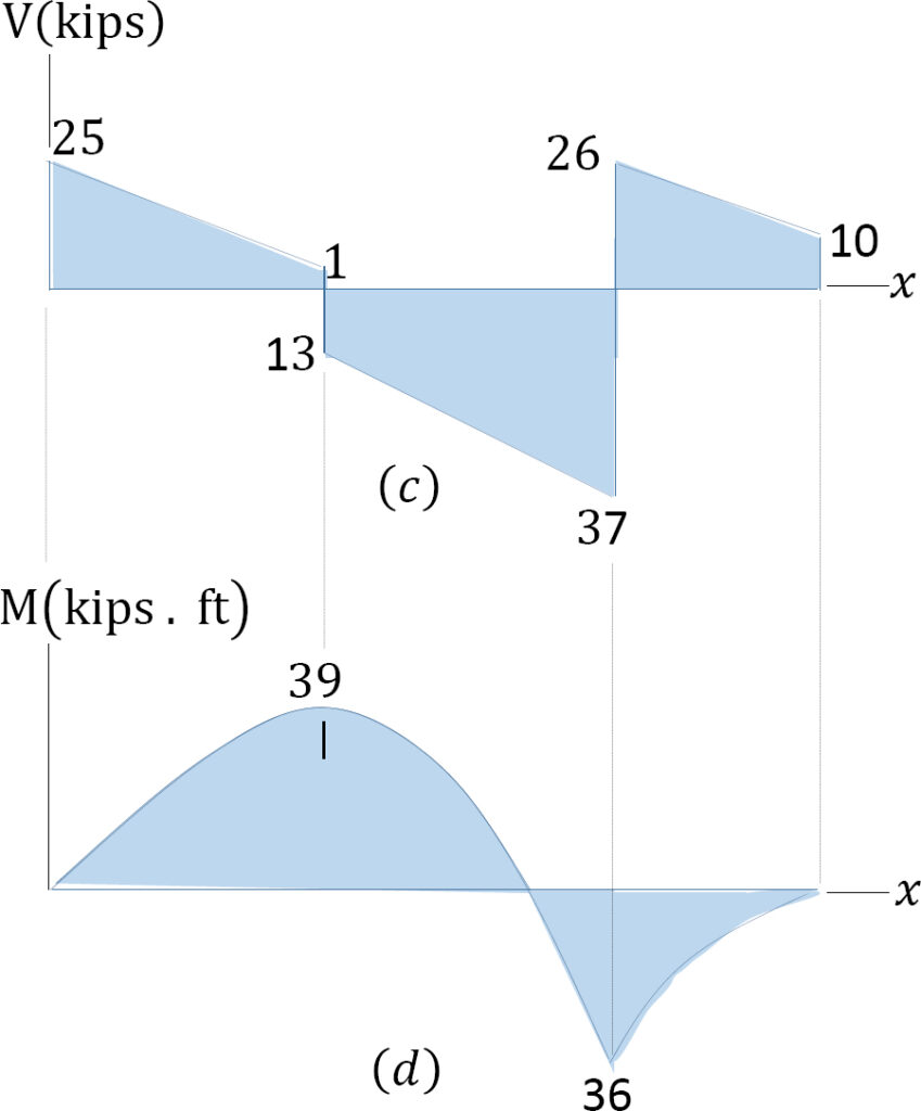
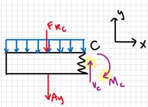
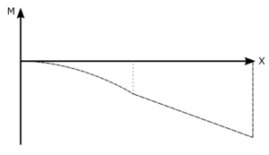
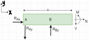
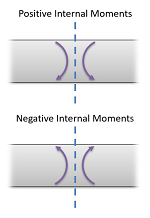 To read the plot, you simply need to take the find the location of interest from the free body diagram above, and read the corresponding value on the y-axis from your plot. Positive internal moments would cause the beam to bow downwards (think a smile shape) negative internal moments will cause the beam to bow upwards (think a frown shape). You can also see the positive and negative internal moments in the figure to the right.


